Economics · Reading 12
Oligopoly
CFA Level I · Economics · Reading 12: The Firm and Market Structures · about 49 min
What you'll learn
- LOS 12.a Determine and interpret breakeven and shutdown points (short and long run) and how economies and diseconomies of scale affect long-run average cost.
- LOS 12.b Describe the characteristics of perfect competition, monopolistic competition, oligopoly and pure monopoly.
- LOS 12.c Explain demand, optimal price and output, and pricing strategy for firms under monopolistic competition, in the short run and the long run.
- LOS 12.d Explain demand, optimal price and output, and pricing strategy under oligopoly: kinked demand, Cournot, Stackelberg, Nash equilibrium, collusion and the dominant firm model.
- LOS 12.e Identify the type of market structure a firm operates in and describe the use and limitations of concentration measures (N-firm concentration ratio and HHI).
Module 12.1
Breakeven, Shutdown, and Scale
This reading explains how a firm decides whether to operate, shut down or change its scale, and how price and output are set under perfect competition, monopolistic competition, oligopoly and monopoly. It ends with the concentration ratio and the Herfindahl-Hirschman Index, the measures used to identify a market structure.
LOS 12.a — Breakeven, shutdown and scale
Short run versus long run
The short run is the period over which at least one factor of production (usually capital: plant and equipment) is fixed, so the firm cannot change its scale. In the long run every input is variable: leases can lapse and equipment can be sold, so no cost is fixed.
Revenue and cost measures
The breakeven and shutdown rules compare revenue with cost, either in totals or per unit of output ():
| Measure | Definition |
|---|---|
| Total revenue (TR) | |
| Average revenue (AR) | , equal to the price when every unit sells at one price |
| Marginal revenue (MR) | Extra revenue from selling one more unit, |
| Total fixed cost (TFC) | Costs that do not change with output in the short run, such as rent under a lease |
| Total variable cost (TVC) | Costs that rise with output, such as materials or merchandise |
| Total cost (TC) | |
| Average variable cost (AVC) | |
| Average total cost (ATC) | |
| Marginal cost (MC) | Extra cost of producing one more unit, |
Breakeven and shutdown for a price taker
A firm in perfect competition is a price taker: it can sell any quantity at the market price, so price = AR = MR.
Key concept
| Condition | Short run | Long run |
|---|---|---|
| Operate (zero or positive economic profit) | Stay in the market | |
| Operate: revenue covers variable cost, so the loss is no larger than fixed cost | Exit (shut down) unless price is expected to rise | |
| Shut down: operating loses more than fixed cost | Exit |
- Breakeven point: (minimum of ATC for a price taker), where and economic profit is zero.
- Short-run shutdown point: minimum of AVC; below it the firm shuts down.
- Long-run shutdown point: minimum of ATC, the same price as the breakeven point; a firm that expects price to stay below ATC leaves the market.
Both shutdown rules ask one question: does revenue cover the costs the firm could avoid by closing? In the short run only variable costs are avoidable, because fixed costs such as a lease must be paid anyway, so price is compared with AVC. In the long run every cost is avoidable, so price is compared with ATC.
MC cuts both AVC and ATC at their lowest points. When the next unit costs less than the current average, producing it pulls the average down; when it costs more, it pulls the average up. The averages therefore fall while MC lies below them and rise once MC is above them. Minimum AVC comes at a smaller output than minimum ATC. The shutdown point therefore sits below and to the left of the breakeven point, both on the MC curve.
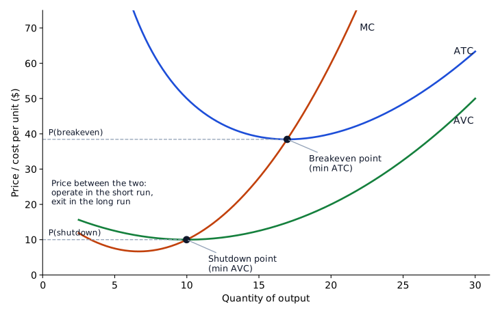
A price taker is too small relative to the market to raise the market price by cutting its own output. Reducing output to push the price up is therefore never a remedy under perfect competition.
Breakeven and shutdown in total terms (all market structures)
For price searchers (downward-sloping demand), price no longer equals MR, so total revenue and total cost are the cleaner test. The same test works for price takers:
- Compare TR with TC. If , the firm stays in the market in both the short run and the long run; is the breakeven point.
- If , compare TR with TVC. If , keep operating in the short run and exit in the long run unless conditions are expected to improve.
- If , shut down now and exit in the long run as well.
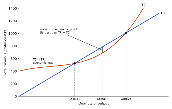
With a straight-line TR (price taker) and a cubic-shaped TC there can be two breakeven quantities. Economic profit is largest where the vertical gap is greatest, which is where the slope of TC (marginal cost) equals the slope of TR (marginal revenue, here the price). At the lower breakeven quantity MC is below MR, so producing more adds profit; at the upper breakeven quantity MC is above MR, so producing less adds profit. If TC lies above TR everywhere, the firm operates (if at all) where the loss is smallest, which is the same as where is largest (least negative).
Worked example. Fernhill Printing expects annual total revenue of $1.8 million, total variable cost of $1.5 million and total fixed cost of $0.5 million, so total cost is $2.0 million. Step 1: , so the firm is not breaking even. Step 2: , so operating gives million, against million (the whole fixed cost) if it closes. It should keep operating in the short run and, unless conditions improve, exit in the long run. If revenue instead fell to $1.3 million, step 3 would apply: , and operating would give million, a loss larger than the fixed cost, so closing at once is the better choice.
Economies and diseconomies of scale
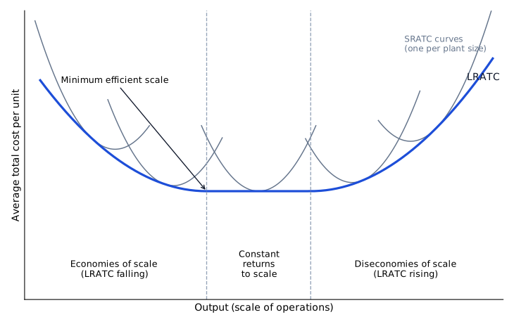
The long-run average total cost (LRATC) curve shows the lowest ATC achievable at each output level when plant size can be chosen freely; it is the envelope of the short-run average total cost (SRATC) curves for the different plant sizes.
| LRATC segment | Name | Causes / meaning |
|---|---|---|
| Downward sloping | Economies of scale (increasing returns to scale) | Specialization of labor, mass production, better equipment and technology, volume discounts on inputs; output rises proportionally more than total input cost |
| Flat | Constant returns to scale | ATC roughly unchanged across a range of plant sizes |
| Upward sloping | Diseconomies of scale | Bureaucracy, harder-to-motivate workforce, barriers to innovation; unit cost rises as scale rises |
The plant size at which LRATC first reaches its lowest level is the minimum efficient scale. Under perfect competition firms must operate there in long-run equilibrium, where price = minimum LRATC and economic profit is zero; a firm that has chosen a scale with higher ATC earns economic losses and must either move to the minimum efficient scale or leave the industry. A firm still in the economies-of-scale range can become more competitive by expanding output and lowering its unit cost. A firm experiencing diseconomies of scale should reduce its plant size (scale) toward the minimum efficient scale. This is a long-run decision, because plant size cannot change in the short run. The US auto industry is a commonly cited case of diseconomies of scale. Economies of scale are a long-run concept: they describe the LRATC curve. The cost curve of a single existing plant cannot show them.
Common exam traps
- The minimum efficient scale is the plant size at the lowest point of LRATC. It is not the largest plant the firm could build.
- The output with the lowest ATC is the cheapest output per unit. It is not necessarily the profit-maximizing output, which is where MR = MC.
- Shutting down "temporarily until price exceeds ATC" is wrong when price is above AVC: it would turn a loss smaller than fixed cost into a loss equal to fixed cost.
Exam shortcuts
- Decide breakeven and shutdown with two comparisons in order: TR against TC, then TR against TVC.
- Short-run shutdown compares price with AVC; long-run exit compares price with ATC.
Bottom line
- In the short run at least one input is fixed; in the long run every input is variable.
- A price taker breaks even at a price equal to minimum ATC and shuts down in the short run when price falls below minimum AVC.
- When price is between AVC and ATC the firm keeps operating in the short run, because its loss is smaller than its fixed cost, and exits in the long run unless price is expected to rise.
- In any market structure: means stay; means operate in the short run and exit in the long run if the shortfall is expected to persist; means shut down.
- Marginal cost crosses AVC and ATC at their minimum points.
- The minimum efficient scale is the lowest point of LRATC; economies of scale make LRATC fall and diseconomies of scale make it rise.
Quick check
Hartwell Joinery employs 35 carpenters and makes furniture in a factory it leases on a five-year contract, using machinery it owns. Over which inputs does the firm have a choice in the long run?
Show answer and explanation
Correct answer: C
The long run is the period over which every factor of production is variable. The firm can let the lease expire or sign a new one, sell or buy machinery and change its workforce, so all three inputs can be changed. In the short run the factory and machinery are fixed and only labor (and materials) can vary.
Why the other options are wrong
- A. Labor alone describes the short run, when the plant and equipment are fixed. In the long run the plant and equipment can be changed as well.
- B. This reverses the usual assumption: labor is variable even in the short run, so it is certainly variable in the long run.
Key takeaway In the long run all costs are variable; the short run is defined by at least one fixed input, usually capital.
Module 12.2
Characteristics of Market Structures
LOS 12.b — The four market structures
Every firm maximizes profit by producing the quantity at which marginal revenue (MR) equals marginal cost (MC). What differs is the demand curve the firm faces. Demand is elastic when buyers react strongly to a price change (a small price rise loses many sales) and inelastic when they react little:
Key concept
- Under perfect competition the firm is a price taker: its demand curve is horizontal (perfectly elastic) at the market price, so .
- Under monopolistic competition, oligopoly and monopoly the firm is a price searcher: its demand curve slopes downward, so and, at the profit-maximizing output, . As a rough rule, monopolistic competitors face relatively elastic demand, a monopolist the least elastic demand, and oligopolists something in between.
Why for a price searcher: to sell one more unit the firm must cut its price, and the lower price applies to every unit it sells, not only to the extra one. MR is the price of the extra unit minus the revenue given up on the units that could have been sold at the higher price.
| Quantity | Price ($) | Total revenue ($) | Marginal revenue ($) |
|---|---|---|---|
| 1 | 50 | 50 | 50 |
| 2 | 46 | 92 | 42 |
| 3 | 42 | 126 | 34 |
| 4 | 38 | 152 | 26 |
| 5 | 34 | 170 | 18 |
| 6 | 30 | 180 | 10 |
Example. In the schedule above, moving from 3 to 4 units lowers the price from $42 to $38. The fourth unit brings in $38, but the first three units now sell for $4 less each, a loss of $12. So , the same as . A price taker faces no such loss: every extra unit sells at the market price, so , and selling 10% more units raises its total revenue by 10%.
Where a market sits on the spectrum depends on five factors: the number and relative size of firms, the degree of product differentiation, the firms' pricing power, barriers to entry and exit, and how much firms compete on things other than price.
| Feature | Perfect competition | Monopolistic competition | Oligopoly | Monopoly |
|---|---|---|---|---|
| Number of sellers | Many | Many | Few | One |
| Barriers to entry | Very low | Low | High | Very high |
| Substitute products | Very good substitutes (identical) | Good substitutes, but differentiated | Good substitutes or differentiated | No good substitutes |
| Nature of competition | Price only | Price, marketing, features | Price, marketing, features | Advertising |
| Pricing power | None | Some | Some to significant | Significant |
| Firm demand curve | Horizontal (perfectly elastic) | Downward sloping, relatively elastic | Downward sloping | Downward sloping (market demand) |
| Long-run economic profit | Zero | Zero | May be positive | May be positive |
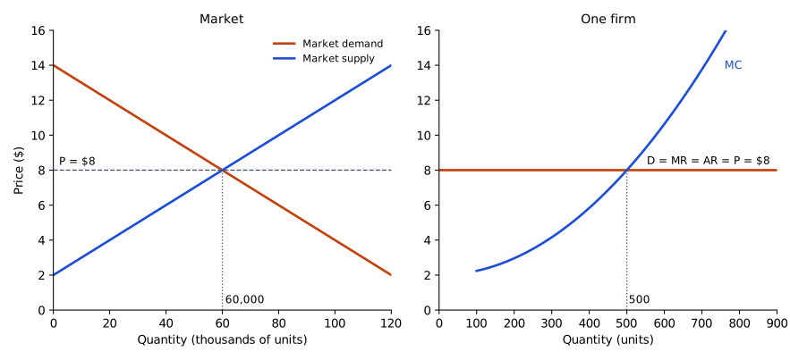
Perfect competition. Many small firms sell identical (homogeneous) products, barriers to entry and exit are very low, and firms compete only on price. No firm can affect the market price; each can sell all it wants at that price, so charging less than the market price simply lowers its revenue. Example: a regional market for a standard grade of grain. The market price comes from market supply and demand, and the market demand curve slopes downward as usual. Each firm takes that price as given, so the demand curve facing the individual firm is horizontal at it.
Monopolistic competition. Many independent sellers, each a price searcher, with differentiated products (quality, features, branding, marketing) and low barriers to entry. Example: toothpaste or restaurants. Heavy advertising is typical.
Oligopoly. A few sellers, each with a large market share; products may be similar or differentiated; high barriers to entry, often due to large economies of scale. The defining feature is interdependence: each firm's best price and output depend on how its rivals will react. Firm demand slopes downward and can be more or less elastic than under monopolistic competition. Examples: automobiles, commercial aircraft, oil.
Monopoly. One firm is the only seller, buyers have no good substitutes for its product, and very high barriers to entry keep rivals out. The barriers can be patents and copyrights, control of a key resource, or government licensing and regulation (e.g., a local utility). The firm faces the market demand curve and has significant pricing power.
Common exam traps
- "Maximizes profit" and "produces where MR = MC" apply to all structures, so they never distinguish one structure from another.
- A vertical demand curve is perfectly inelastic, the opposite of the perfectly competitive firm's horizontal curve.
- Barriers to entry under monopolistic competition are low: neither absent altogether nor high.
- Advertising and product differentiation separate monopolistic competition from perfect competition; low barriers and zero long-run economic profit are common to both.
LOS 12.c — Monopolistic competition: price, output and strategy
Features that drive behavior:
- Many independent sellers. Each firm's share is small, so no firm has significant power over price; firms watch the average market price rather than individual rivals' prices; there are too many firms for collusion (price-fixing) to work.
- Differentiated products that are close substitutes. Firms compete more on quality, features and marketing than on price. Because close substitutes exist, firm demand is relatively elastic: a firm that raises its price loses many customers.
- Low barriers to entry: because entering and exiting cost little, new firms arrive whenever existing firms earn economic profit.
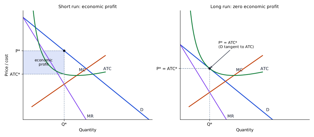
Short run. The firm sets its price and output in three steps (left panel below):
- Find the output at which .
- Go up from to the demand curve and read off the price that buyers will pay for that quantity.
- Compare with ATC at . Economic profit is , positive when price exceeds ATC and negative when it falls short.
Long run. Low barriers attract entrants, and each existing firm's demand shifts left until it is just tangent to ATC: and economic profit is zero (right panel). The same outcome can arise without entry if firms keep raising marketing spending (part of ATC) to defend market share. Accounting profit can stay positive even while economic profit is driven to zero.
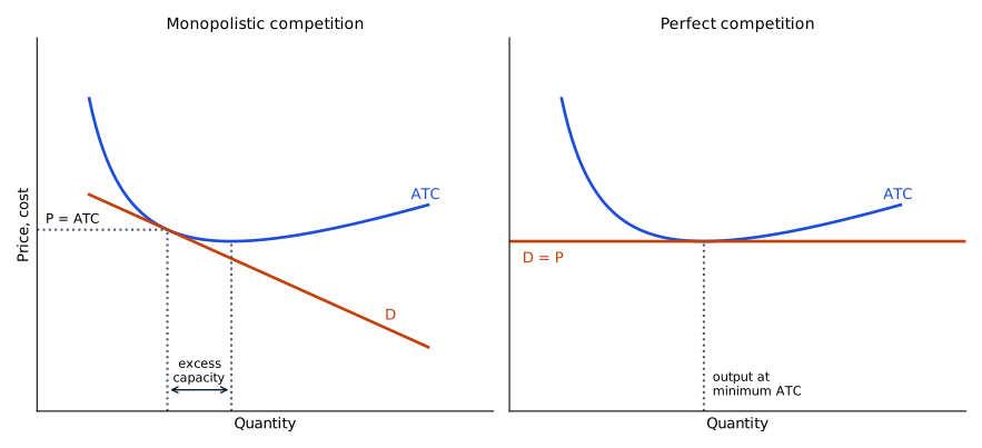
Long-run comparison with perfect competition: in monopolistic competition , ATC is not at its minimum (excess capacity), price is higher and quantity lower. The offset is product variety, which consumers value.
Product differentiation and brands. The fewer close substitutes buyers see for a product, the steeper (less elastic) its demand curve. A medicine that some patients tolerate better than its rivals faces steeper demand than one brand of shampoo among many, and a new product with no close rival is in the same position. Brand names can signal quality and help consumers choose. There is no well-defined firm supply curve.
Worked example. A craft-coffee roaster sells 5,000 bags a month at $14 while its ATC is $11: economic profit . New roasters enter; the roaster's demand shifts left until, at its new MR = MC output, price equals ATC (for example, both at $12.50) and economic profit is zero.
Common exam traps
- Reading the price off the MR or MC curve at understates it: both lie below the demand curve there, because for a price searcher.
LOS 12.d — Oligopoly: interdependence and pricing models
Because oligopolists are interdependent, a price change by one firm is likely to trigger a response that shifts the others' demand curves. The optimal price therefore depends on what a firm assumes about its rivals' reactions. Four models:
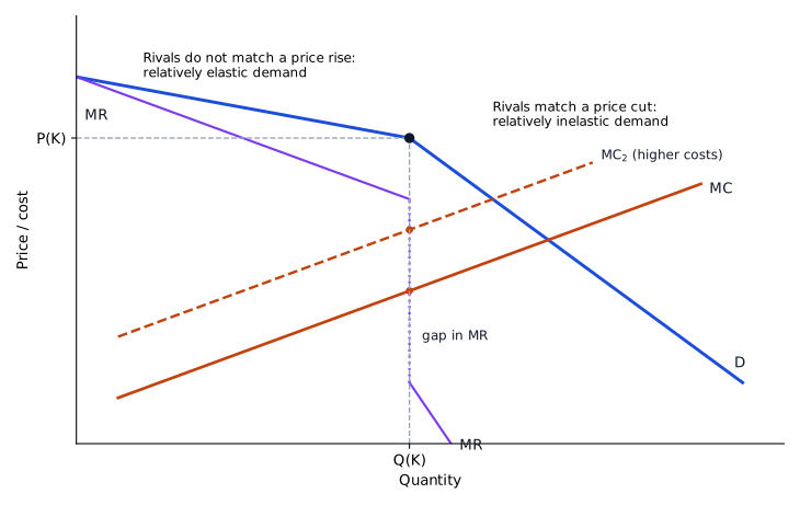
1. Kinked demand curve model. Rivals are assumed not to match a price increase but to match a price cut. The firm's demand curve is therefore relatively elastic above the current price and relatively inelastic below it, creating a kink at . Each segment of demand has its own MR curve, and the MR of the steep lower segment starts well below the MR of the flat upper segment, so MR drops straight down at and leaves a gap. Any MC curve passing through the gap leaves the profit-maximizing price at and output at . A rise in costs that keeps MC inside the gap (from MC to in the figure) therefore leaves price and output unchanged, so prices tend to be sticky. Only a cost change that pushes MC above or below the gap moves them.
2. Cournot duopoly model. Two firms with identical MC curves selling a homogeneous product; each chooses its output (quantity) assuming the competitor's output will not change, and the firms choose simultaneously each period. The market price is whatever single price clears the combined output. In the long-run equilibrium both firms sell the same quantity and split the market equally, at a price below the monopoly price but above the perfectly competitive price. With more firms, the price moves toward the competitive price.
3. Stackelberg model (the Stackelberg dominant firm model). Decisions are sequential: the leader chooses its output first and the follower then chooses its own output in response. The leader exploits this first-mover advantage to produce the larger quantity and so gains the larger market share and the larger share of total profits, even in the long run. Both firms still sell the homogeneous product at one common market price; the leader does not charge a different price from the follower.
Exam convention: both models are described with each firm choosing its selling price; a Cournot firm assumes the rival keeps last period's price, and the Stackelberg leader sets its price first, charges a higher price and earns the larger share of total profit. Current practice: both are the quantity-setting models described above, with one market price. Both are rules-based models and fall under strategic games, decision models in which a firm's best choice depends on rivals' expected actions.
4. Nash equilibrium. A Nash equilibrium is reached when no firm can improve its profit by unilaterally changing its choice, given the others' choices. The Cournot outcome is a Nash equilibrium. Absent collusion, the long-run oligopoly equilibrium is a Nash equilibrium.
To find a Nash equilibrium in a payoff table:
- For each choice the rival could make, mark the firm's best reply, meaning the choice that earns the firm more.
- Repeat for the rival, taking each of the firm's choices in turn.
- A cell in which both choices are marked is a Nash equilibrium.
Worked example. Kestrel and Osprey each choose a high or low price; payoffs are shown below. Step 1: if Osprey prices high, Kestrel's best reply is low (850 > 700); if Osprey prices low, it is low again (400 > 250). Step 2: the payoffs are symmetric, so Osprey's best reply is also low whatever Kestrel does. Step 3: only (low, low) has both choices marked, so it is the Nash equilibrium, with 400 each, even though (high, high) would give both 700.
| Osprey: high price | Osprey: low price | |
|---|---|---|
| Kestrel: high price | Kestrel 700, Osprey 700 | Kestrel 250, Osprey 850 |
| Kestrel: low price | Kestrel 850, Osprey 250 | Kestrel 400, Osprey 400 |
Collusion. Collusion is an agreement among competitors to charge a given price or to limit output to agreed levels. If the firms could agree on (and enforce) high prices, both would earn more; side payments can make the collusive outcome better for each firm than the Nash equilibrium. That is the incentive behind a cartel such as OPEC, whose members agree to restrict output to raise price. Members have an incentive to cheat by producing more. Collusion is more likely to hold when there are fewer firms, products are more similar, cost structures are more similar, purchases are small and frequent, retaliation against cheaters is more certain and severe, and there is little competition from outside the cartel. Such agreements are illegal in many countries.
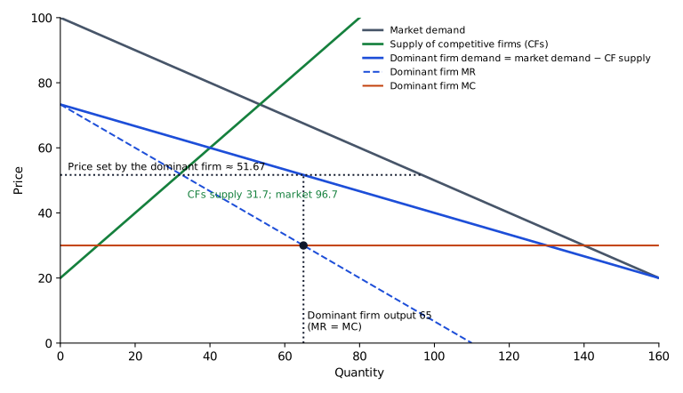
Dominant firm model. One firm with a large market share, owing to its greater scale and lower cost structure, effectively sets the market price; the smaller competitive firms (CFs) take that price as given and produce where their MC equals it. The dominant firm's demand curve is market demand minus the CFs' supply (the CFs supply less at lower prices); the dominant firm sets price where its own MR equals its MC. If CFs cut price, the dominant firm follows; in the long run the CFs reduce output or exit, and the dominant firm's market share rises.
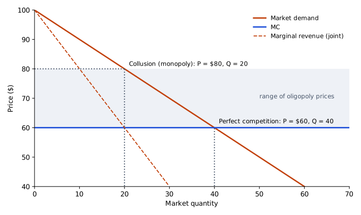
Range of outcomes. Oligopoly price lies between two limits: the collusion (monopoly) price that maximizes joint profit, and the perfectly competitive price that yields zero economic profit. Example: if the joint-profit-maximizing price is $80 and the competitive price is $60, the oligopoly price should be somewhere in between, e.g. about $70, and neither above $80 nor below $60.
As in monopolistic competition, in equilibrium, there is no well-defined supply curve, and economic profit may be positive in the long run, though it may erode over time.
Common exam traps
- Cournot and Stackelberg differ in timing (simultaneous versus sequential choices). Both are strategic-game (rules-based) models, so that is not a difference between them.
- An option that cites many sellers or low barriers to entry does not describe an oligopoly.
- A Nash equilibrium need not maximize joint profit; the collusive outcome usually earns more.
Exam shortcuts
- Classify a market from two facts first: the number of firms and the barriers to entry. Many firms with identical products is perfect competition; many with differentiated products and low barriers is monopolistic competition; a few interdependent firms behind high barriers is oligopoly; one firm with no close substitutes is monopoly.
- To find a Nash equilibrium, mark each player's best reply to every choice of the rival; a cell with both choices marked is an equilibrium.
- Under the kinked demand curve model, a cost change that keeps MC inside the gap in MR leaves price and output unchanged.
Bottom line
- Every firm maximizes profit where MR = MC; a price taker has , while a price searcher has .
- Monopolistic competition has many firms, differentiated products and low barriers, and earns zero economic profit in the long run with excess capacity.
- Oligopoly is defined by interdependence among a few large firms protected by high barriers to entry.
- Cournot firms decide simultaneously and the Stackelberg leader decides first; exam convention: they choose prices, the Cournot firm assuming its rival keeps last period's price and the Stackelberg leader charging a higher price and earning the larger share of total profit; current practice: they choose quantities and sell at one market price.
- In a Nash equilibrium no firm can gain by changing its choice alone, and the outcome need not maximize joint profit.
- The oligopoly price lies between the collusive (monopoly) price and the perfectly competitive price.
Quick check
An industry study reports the following:
- many sellers act independently of one another;
- product features differ from firm to firm;
- entry into the industry is easy;
- each firm's demand curve slopes downward but is quite elastic.
The industry is best characterized as:
Show answer and explanation
Correct answer: B
Many independent sellers, differentiated products, low barriers to entry and downward-sloping, highly elastic firm demand are the conditions of monopolistic competition.
Why the other options are wrong
- A. An oligopoly has a small number of interdependent sellers and high barriers to entry.
- C. A monopoly has a single seller protected by high barriers to entry.
Key takeaway Checklist for monopolistic competition: many sellers, differentiation, easy entry, elastic downward-sloping demand.
Module 12.3
Identifying Market Structures
LOS 12.e — Identifying the market structure and measuring concentration
Identifying the structure
To classify the market a firm operates in, compare the industry with the characteristics of each structure (see the comparison table in Module 12.2): the number of firms and their relative sizes, the barriers to entry, the nature of substitute products (identical, differentiated, none), and the nature of competition (price only versus marketing and features). For an analyst trying to gauge pricing power, these are the factors that matter. Significant interdependence in pricing and output is present in every oligopoly, and some interdependence can appear even under monopolistic competition.
Classifying a market does not, however, show how much pricing power each firm has. The ideal would be to measure the elasticity of firm demand directly, but that is statistically difficult and imprecise. Regulators and analysts therefore use measures based on market shares, called concentration measures, as a proxy for market power and to help identify the market structure. Competition authorities often block mergers when the combined firm's share would be too high.
The two concentration measures
| Measure | Calculation | Strength | Weakness |
|---|---|---|---|
| N-firm concentration ratio | Sum of the percentage market shares of the largest N firms | Simple to compute and interpret | Relatively insensitive to mergers among the largest firms; does not measure market power or elasticity directly |
| Herfindahl-Hirschman Index (HHI) | Sum of the squared market shares of the largest N firms | Squaring gives big firms more weight, so it is more sensitive to mergers | Still does not measure market power directly |
Key concept
where is firm 's market share as a decimal. With shares in percent, the HHI is expressed on a 0 to 10,000 scale. A market served by one firm has a concentration ratio of 100% and an HHI of 1 (10,000 in percent terms), the highest possible values.
To compute either measure:
- Rank the firms by market share and keep the N largest. If the data are sales rather than shares, first divide each firm's sales by total industry sales, including the sales of all the smaller firms.
- For the concentration ratio, add their shares. For the HHI, square each share and add the squares.
- To assess a merger, combine the merging firms' shares into one firm, re-rank all the firms and repeat steps 1 and 2. The list of the N largest can change: the merged firm may move up the ranking, and if two of the top N firms merge, the next-largest firm moves into the top N.
Worked example. Market shares are shown below. Two of the top five firms, Dunmore and Easton, plan to merge.
| Firm | Market share |
|---|---|
| Ashby | 28% |
| Brennan | 22% |
| Corlett | 16% |
| Dunmore | 10% |
| Easton | 8% |
| All others (each below 5%) | 16% |
Before the merger: 4-firm ratio ; 4-firm HHI .
After the merger the combined firm has 18%, and the top four are 28%, 22%, 18%, 16%: 4-firm ratio ; 4-firm HHI .
Limitations common to both measures
- Neither considers barriers to entry or potential competition. Firms with large market shares may still have little pricing power if entry is easy: would-be entrants stand ready to come in if incumbents raise prices, so firm demand can be quite elastic despite high concentration. A few firms making an easily copied product with no brand or patent protection may therefore behave much like perfectly competitive firms.
- Neither measures the elasticity of firm demand (market power) directly.
Common exam traps
- Mixing scales: an HHI of 0.1624 (shares as decimals) is the same as 1,624 (shares in percent).
- Reading a small rise in the N-firm ratio after a merger as a small rise in concentration. When two of the top N firms combine, the ratio grows only by the share of the firm that enters the top N, while the HHI can rise sharply.
Exam shortcuts
- With shares in whole percentages, square and add them to get the HHI on the 0 to 10,000 scale without converting to decimals.
- When two of the top N firms merge, the N-firm concentration ratio rises only by the share of the firm that enters the top N.
Bottom line
- A market structure is identified by the number of firms, the barriers to entry, the nature of substitutes and the nature of competition.
- The N-firm concentration ratio is the sum of the N largest market shares; the HHI is the sum of their squared shares.
- The HHI is more sensitive than the concentration ratio to mergers among the largest firms.
- Neither measure accounts for barriers to entry or potential competition, and neither measures the elasticity of firm demand directly.
Quick check
An analyst has annual sales for the producers of industrial fasteners in a region:
| Firm | Sales (€ millions) |
|---|---|
| Arlo | 240 |
| Brisk | 180 |
| Calder | 150 |
| Dunmark | 120 |
| Eske | 60 |
| All other firms | 50 |
The industry's three-firm concentration ratio and three-firm Herfindahl-Hirschman Index (HHI) are closest to:
Show answer and explanation
Correct answer: A
Both measures use market shares, so each firm's sales must first be divided by total industry sales, including the sales of all the smaller firms. The three-firm concentration ratio adds the shares of the three largest firms; the three-firm HHI adds the squares of those shares.
Total industry sales .
Shares of the three largest firms: , , .
Why the other options are wrong
- B. 0.1983 also squares Dunmark's 15% share (), which is a four-firm HHI. The question asks for the three largest firms only.
- C. These values leave the other firms' sales of 50 out of the total, so shares are computed on 750: and .
Key takeaway Convert sales to shares using total industry sales, then use the same N largest firms for both measures.
Practice Questions
Lindqvist Ferries operates in a market in which it faces a downward-sloping demand curve. For the coming year it forecasts total revenue of $2.10 million, total variable costs of $1.65 million and total fixed costs of $0.72 million. If these conditions are expected to persist, the firm should most appropriately:
Show answer and explanation
Correct answer: B
For a price searcher, breakeven and shutdown are judged with totals because price does not equal marginal revenue. Total revenue exceeds total variable cost, so operating covers all variable cost and part of fixed cost and loses less than shutting down; but total revenue is below total cost, so the firm cannot survive in the long run when all costs are avoidable.
Total cost: million.
- Loss if it operates: million.
- Loss if it shuts down (fixed costs still due): million.
Since : operate in the short run (a loss of $0.27 million instead of $0.72 million), but exit in the long run because TR does not cover TC.
Why the other options are wrong
- A. Short-run shutdown is warranted only when . Here TR exceeds TVC by $0.45 million, so closing now would raise the loss from $0.27 million to the full $0.72 million of fixed costs.
- C. Covering variable costs is enough only for the short run. In the long run the firm must cover total cost; with TR below TC by $0.27 million it should exit if conditions persist.
Key takeaway If , shut down now; if , operate now and exit later; if , stay.
Norden Cement and Solvik Cement are the only two suppliers in a regional market. Each firm independently chooses a high or a low price, and the resulting annual profits are shown below.
| Solvik: high price | Solvik: low price | |
|---|---|---|
| Norden: high price | Norden 800, Solvik 700 | Norden 300, Solvik 900 |
| Norden: low price | Norden 950, Solvik 250 | Norden 500, Solvik 450 |
Based on the concept of a Nash equilibrium, the most likely outcome is that:
Show answer and explanation
Correct answer: B
A Nash equilibrium is a combination of choices from which no firm can raise its profit by changing its own choice alone. Charging a low price is each firm's best response whatever the other does, so both choose a low price and neither wants to deviate, even though both would earn more if they could collude on high prices.
Norden's best response: if Solvik is high, low (950) beats high (800); if Solvik is low, low (500) beats high (300), so Norden prices low either way.
Solvik's best response: if Norden is high, low (900) beats high (700); if Norden is low, low (450) beats high (250), so Solvik prices low either way.
Nash equilibrium: (low, low) with profits 500 and 450. Joint profit there is 950 versus 1,500 at (high, high), the collusive outcome.
Why the other options are wrong
- A. Both charging high gives the largest joint profit (1,500), but it is not stable: either firm could raise its own profit by switching to a low price (Norden from 800 to 950, Solvik from 700 to 900). Only collusion could sustain it.
- C. If Solvik prices low, Norden earns only 300 with a high price versus 500 with a low price, so Norden would switch; this combination is not an equilibrium.
Key takeaway Check each cell: if either firm can gain by changing only its own choice, the cell is not a Nash equilibrium. The Nash equilibrium need not maximize joint profit.
This reading has 65 questions in the full bank. Practice all of them.
Key Takeaways
- In the long run all costs are variable; the short run is defined by at least one fixed input, usually capital.
- If , shut down now; if , operate now and exit later; if , stay.
- Checklist for monopolistic competition: many sellers, differentiation, easy entry, elastic downward-sloping demand.
- Check each cell: if either firm can gain by changing only its own choice, the cell is not a Nash equilibrium. The Nash equilibrium need not maximize joint profit.
- Convert sales to shares using total industry sales, then use the same N largest firms for both measures.