Equities · Reading 44

Discounted Cash Flow (DCF) and Growth Models

CFA Level I · Equities · Reading 44 · about 51 min

Equities notes as a PDF125 pages · 1.8 MB · free, no sign-up · All PDFs

What you'll learn

LOS 44.a Contrast the inputs of dividend, FCFE, FCFF and residual income models (and EBITDA as a proxy) and explain the five-step process for valuing equity with present value models.
LOS 44.b Calculate and interpret intrinsic value with constant growth and multistage present value models, including sustainable growth, implied growth, and FCFF discounted at the WACC.
LOS 44.c Explain the shortcomings of constant and multistage growth assumptions in present value models.
LOS 44.d Value non-callable, non-convertible preferred stock (finite and perpetual) and explain how callable, putable and convertible features change its value.

Module 44.1

Cash Flow Metrics

This reading covers the cash flow measures used in present value models (dividends, FCFE, FCFF, EBITDA and residual income) and the steps of the valuation process. It shows how to value shares with constant growth and multistage models, how to estimate growth and the WACC, where growth assumptions fall short, and how to value preferred stock and judge the effect of call, put and conversion features.

LOS 44.a — Cash flow measures for present value models and the valuation process

A present value model (also called a discounted cash flow (DCF) model) values equity as the present value of the cash flows shareholders can expect. Unlike a fixed-coupon bond, a common share has no promised cash flows and no maturity date, so the analyst must (1) forecast a cash flow measure over a forecast horizon and (2) estimate a terminal value that captures everything beyond the horizon. Value today is the present value of both:

V_{0} = t = 1 \sum n \frac{E ( C F _{t} )}{( 1 + r ) ^{t}} + \frac{E ( T V _{n} )}{( 1 + r ) ^{n}}

where $n$ is the number of periods in the forecast horizon and $r$ is the discount rate that matches the cash flow measure.

Five measures are used. Two of them, EBITDA and residual income, are not cash flows, yet the same discounting framework still applies to them.

Key concept

Measure	What it represents	Perspective	Discount rate	Works best when
Dividends	Cash actually paid to shareholders	Minority shareholder (cannot set dividend policy)	Required rate of return on equity	Positive, stable/growing earnings; high, consistent payout; stable capital structure and share count
Free cash flow to equity (FCFE)	Cash that could be paid to common shareholders: the firm's capacity to pay dividends	Controlling shareholder	Required rate of return on equity	Non-payers or firms whose payout differs from capacity; stable capital structure
Free cash flow to the firm (FCFF)	Cash from operations, before interest, left after the investment needed to sustain capacity; available to debt and equity holders	Whole firm / all capital providers (pre-leverage)	Weighted average cost of capital (WACC)	High capital spending (negative FCFE) or a volatile capital structure
EBITDA	Pre-tax, pre-leverage earnings	Pre-leverage	WACC, as for FCFF	Rough proxy only; needs adjusting to reach FCFF
Residual income	Earnings in excess of the cost of equity (economic profit)	Equity	Required rate of return on equity	FCFE and FCFF negative with no clear date for turning positive

Dividends

Dividend discount models (DDMs) use the dividends shareholders expect to receive. They are theoretically justified because dividends are the cash equity investors actually get. The model assumes earnings are either paid out or retained to fund growth; if the firm borrows to pay dividends or buy back stock (i.e., changes its capital structure), that assumption breaks and a DDM is a poor choice. DDMs suit mature payers and industries where high payouts are required by law or regulation (e.g., REITs, regulated utilities). Drawbacks: hard to apply to non-dividend-paying firms, and they reflect only a minority holder's view.

Free cash flow to equity

FCFE is the cash left for common shareholders after the firm pays its debt obligations and funds the working capital and capital expenditures needed to maintain existing assets and grow:

Key concept

F C F E = net income + depreciation - W C I n v - C a pE x + net borrowing

F C F E = C F O - F C I n v + net borrowing

WCInv is investment in working capital and CapEx is capital expenditure, which the second form calls fixed capital investment (FCInv). Net income plus depreciation minus WCInv approximates cash flow from operations (CFO), which gives the second form. Net borrowing = new debt borrowed − debt repaid; it is the part of capital spending and working capital investment financed with debt. From the cash flow statement, FCFE can also be read as its uses: $F C F E = Δ cash + dividends - Δ equity$ , where $Δ equity$ = shares issued − shares repurchased. In other words, FCFE can be used to add to cash, pay dividends or buy back shares.

If the firm keeps a target debt-to-assets ratio (DR), it borrows DR of every dollar of net investment:

net investment = C a pE x - depreciation + W C I n v

F C F E = net income - net investment + net borrowing, net borrowing = D R \times net investment

F C F E = net income - net investment + D R \times net investment = net income - (1 - D R) (net investment)

Free cash flow to the firm

FCFE is less useful when heavy capital spending makes it negative or when the capital structure is volatile (future borrowing is hard to forecast). Then use FCFF, a pre-leverage cash flow:

F C F F = C F O - C a pE x + interest (1 - t)

F C F F = F C F E + interest (1 - t) - net borrowing

Here t is the tax rate. Only after-tax interest is added back because interest reduces taxes. For a firm with no debt, FCFF = FCFE.

EBITDA

EBITDA differs from FCFF because it is before tax, ignores the tax savings on depreciation, and ignores investment in fixed and working capital:

F C F F = E B I T D A (1 - t) + (depreciation \times t) - F C I n v - W C I n v

"Adjusted EBITDA" figures remove items management calls non-recurring; the adjustments are subjective and not an accounting-standard measure.

Residual income

Residual income = net income minus a charge for the cost of equity capital. Per share:

R I_{t} = E P S_{t} - r \times B V P S_{t - 1}

It is discounted at the required return on equity. The model requires clean surplus accounting: book value of equity changes only through the income statement (retained earnings) and transactions with shareholders (dividends, issuance, buybacks). Items that bypass the income statement (e.g., foreign currency translation gains/losses) must be adjusted for.

The valuation process

Choose the cash flow measure.
Forecast it over a horizon suited to the company.
Choose the discount rate consistent with that measure.
Estimate a terminal value for the period beyond the horizon.
Compute the present values of the forecast cash flows and terminal value and add them.

Worked example

Lindqvist Marine reports net income 80, depreciation 25, working capital investment 10, capital expenditures 45, net borrowing 12, interest expense 15, tax rate 30% (all in millions).

$F C F E = 80 + 25 - 10 - 45 + 12 = 62$
$F C F F = 62 + 15 (1 - 0.30) - 12 = 60.5$

A share with EPS of 3.00 this year, beginning book value per share of 20.00 and a 10% required return earns $R I = 3.00 - 0.10 \times 20.00 = 1.00$ per share.

Common exam traps

Match measure and rate: the cost of equity is the rate for dividends, FCFE and residual income, and the WACC is the rate for FCFF. FCFE is never discounted at a cost of debt, nor residual income at the WACC.
A DDM takes a minority-shareholder view; FCFE takes a controlling-shareholder view, while FCFF takes the whole-firm view. FCFE is the capacity to pay; dividends are what is actually paid.
Net borrowing is added in FCFE and subtracted when moving from FCFE to FCFF. In the worked example, adding the 12 of net borrowing again when moving to FCFF gives 84.5 instead of 60.5.
With a target DR, multiply net investment by $(1 - D R)$ rather than by DR.
In the EBITDA bridge, the depreciation tax shield is added.
Calculating the terminal value is step 4; summing present values is the final step.

Exam shortcuts

For a firm with no debt, FCFF equals FCFE, so there is no interest or net borrowing adjustment to make.

Bottom line

A present value model values equity as the present value of a cash flow measure forecast over a horizon plus the present value of a terminal value, using a discount rate that matches the measure.
A DDM takes the minority shareholder's view and suits mature firms with high, consistent payouts, while FCFE, the capacity to pay dividends, takes a controlling shareholder's view; the discount rate for both is the required return on equity.
$F C F E = net income + depreciation - W C I n v - C a pE x + net borrowing$ , and with a target debt-to-assets ratio DR it becomes $net income - (1 - D R) (net investment)$ .
FCFF is a pre-leverage cash flow, $F C F F = F C F E + interest (1 - t) - net borrowing$ , discounted at the WACC and used when heavy capital spending makes FCFE negative or the capital structure is volatile.
Residual income per share is $E P S_{t} - r \times B V P S_{t - 1}$ , discounted at the required return on equity, and the model requires clean surplus accounting.
The valuation process chooses the cash flow measure, forecasts it, chooses a matching discount rate, estimates the terminal value and finally sums the present values.

Quick check

Question 1Core

Which of the following statements most accurately contrasts a dividend discount model (DDM) with a free cash flow to equity (FCFE) model?

Show answer and explanation

Correct answer: B

Dividends are what every shareholder receives and reflect the position of an investor who cannot influence dividend policy, which is a minority shareholder perspective. An FCFE valuation reflects a controlling shareholder, who can decide how much of the free cash flow is paid out.

Why the other options are wrong

A. This reverses the two models: the DDM uses the cash actually received (dividends), while FCFE represents the firm's theoretical capacity to pay dividends.
C. Neither model assumes a volatile capital structure or heavy borrowing; each is built on the premise that the firm's financing mix stays steady. When the mix is volatile, FCFF is the preferred measure.

Key takeaway A DDM takes the minority view of cash actually paid; FCFE takes the controlling view of cash that could be paid. Both assume a stable capital structure.

Module 44.2

Valuation Models

LOS 44.b — Constant growth and multistage present value models

Growth and the company life cycle

Start-up: earnings negative and many firms fail, so cash flow models are unsuitable.
Growth: earnings turn positive and grow rapidly; the analyst estimates how long this phase lasts.
Mature: growth settles at a long-run rate in line with the overall economy (multinationals may exceed domestic growth). A constant growth assumption is most plausible here.
Decline: obsolete products or technology.

The best candidates for a constant growth model are (1) mature firms (2) with stable leverage near the industry average and (3) a high dividend payout ratio. A constant rate is also used for the terminal value after a high-growth period.

Constant growth (Gordon growth) model

A share is worth the present value of all its future dividends. If the dividend grows at the same rate g every year and g is below the required return r, that endless sum collapses into one short fraction:

Key concept

V_{0} = \frac{D _{1}}{r - g} = \frac{D _{0} ( 1 + g )}{r - g}

The same form works for FCFE ( $V_{0} = F C F E_{1} / (r - g)$ ) and FCFF (firm value $= F C F F_{1} / (W A C C - g)$ ). Conditions: $g < r$ , and g should be less than the long-run growth rate of the economy. The first condition keeps the value finite. Each dividend's present value is the previous one's multiplied by $(1 + g) / (1 + r)$ , so the present values shrink toward zero only when g is below r; with $g \geq r$ they never shrink and the sum has no finite value.

Past vs expected dividend: "just paid", "last paid" or "currently pays" means $D_{0}$ ; grow it one period. "Will pay next year" or "is expected to pay" means $D_{1}$ ; do not grow it.
Value at a future date: $V_{t} = D_{t + 1} / (r - g) = V_{0} (1 + g)^{t}$ . The model always gives value one period before the dividend in the numerator.
Sensitivity: value rises when r falls or g rises, because the spread $r - g$ in the denominator shrinks.
One-period model: for a one-year holding, the terminal value is the expected price in one year, so $V_{0} = (D_{1} + P_{1}) / (1 + r)$ . If the market price exceeds this value, the share is overvalued; if it is below, undervalued.

Implied growth rate. If the constant growth model fits the company, rearranging it with the market price gives the growth rate the market is pricing in (the same works with $F C F E_{1}$ in place of $D_{1}$ ):

g = r - \frac{D _{1}}{P _{0}}

Multistage (two-stage) models

Two types: (1) growth of $g_{S}$ for n periods, then a perpetual rate $g_{L}$ (usually $g_{S} > g_{L}$ ); (2) cash flows forecast individually for n periods (spreadsheet), then a constant-growth terminal value.

Key concept

V_{0} = t = 1 \sum n \frac{D _{t}}{( 1 + r ) ^{t}} + \frac{V _{n}}{( 1 + r ) ^{n}}, V_{n} = \frac{D _{n + 1}}{r - g _{L}}

Steps: (1) forecast each high-growth dividend; (2) find the first constant-growth dividend $D_{n + 1}$ ; (3) compute the terminal value $V_{n}$ ; (4) discount every dividend and $V_{n}$ at r.

First dividend in the future: if the first dividend $D_{k}$ arrives at the end of year k, the Gordon model gives $V_{k - 1} = D_{k} / (r - g)$ , which is discounted back k − 1 years.

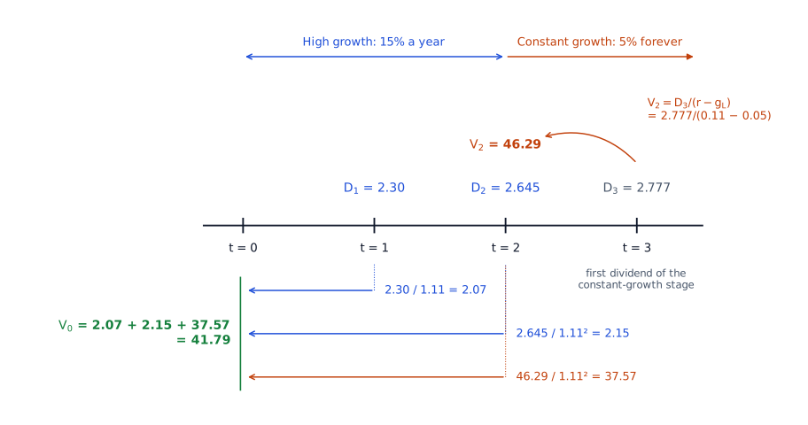
Worked example. $D_{0} = 2.00$ ; growth 15% for two years, then 5% forever; $r = 11%$ .

$D_{1} = 2.30$ , $D_{2} = 2.645$ , $D_{3} = 2.645 \times 1.05 = 2.777$
$V_{2} = 2.777/ (0.11 - 0.05) = 46.29$
$V_{0} = 2.30/1.11 + (2.645 + 46.29) /1.1 1^{2} = 2.07 + 39.72 = 41.79$

Calculator: CF0 = 0; C01 = 2.30; C02 = 48.93; [NPV] I = 11, [↓] [CPT] = 41.79.

The timeline shows the same cash flows and their present values.

Timeline from t = 0 to t = 3. High growth of 15% a year runs from t = 0 to t = 2, then constant growth of 5% forever. D1 = 2.30 at t = 1 and D2 = 2.645 at t = 2. D3 = 2.777 at t = 3 is the first dividend of the constant-growth stage and gives the terminal value V2 = 2.777/(0.11 - 0.05) = 46.29, placed at t = 2. Present values at t = 0: 2.30/1.11 = 2.07; 2.645/1.11 squared = 2.15; 46.29/1.11 squared = 37.57. V0 = 2.07 + 2.15 + 37.57 = 41.79. — Two-stage dividend discount model on a timeline (dividend just paid 2.00; 15% growth for two years, then 5%; required return 11%)

Estimating the constant growth rate

Either use historical growth, which is unreliable if capital structure, margins, competitive position or technology change, or estimate the sustainable growth rate from fundamentals, assuming constant ROE, constant payout and no new equity:

Key concept

g = (1 - dividend payout ratio) \times R O E = b \times R O E

where the retention ratio $b = 1 - payout ratio$ and ROE is measured on beginning book value, so equivalently $g = (1 - dividends / net income) \times (net income / beginning book value)$ . The required return and beta are not inputs. Example: with ROE of 14% and a payout of 60%, $g = 0.40 \times 14% = 5.6%$ . A result far above long-run economic growth should be questioned.

Putting the pieces together, each input of the constant growth model comes from a different place. The table uses one set of illustrative figures.

Where the inputs of the constant growth model come from (illustrative figures)

Input	How it is estimated	Illustration
Dividend just paid, $D_{0}$	Payout ratio × EPS	$0.50 \times 3.00 = 1.50$
Growth rate, g	Sustainable growth: retention ratio × ROE	$0.50 \times 10% = 5%$
Next dividend, $D_{1}$	$D_{0} (1 + g)$	$1.50 \times 1.05 = 1.575$
Required return, r	CAPM: $R_{f} + β [E (R_{m}) - R_{f}]$ (Reading 50)	$3% + 1.2 \times 5% = 9%$
Value, $V_{0}$	$D_{1} / (r - g)$	$1.575/ (0.09 - 0.05) = 39.38$

For FCFE and FCFF:

S G R_{F C F E} = (1 - \frac{F C F E}{net income}) (\frac{net income}{beginning book value})

S G R_{F C F F} = (1 - \frac{F C F F}{N O P A T}) (\frac{N O P A T}{beginning book value of total capital})

with NOPAT = operating income × (1 − t). In theory all three rates agree; in practice they differ and the assumptions must be reconciled.

Weighted average cost of capital

FCFF goes to all capital providers, so its discount rate is the weighted average cost of capital (WACC): the after-tax cost of debt and the cost of equity weighted by their market values.

W A C C = \frac{M V _{d}}{M V _{d} + M V _{e}} r_{d} (1 - t) + \frac{M V _{e}}{M V _{d} + M V _{e}} r_{e}

Debt has priority, so $r_{d} < r_{e}$ . Present value of FCFF = firm value; equity value = firm value − market value of debt; divide by shares outstanding for a per-share value.

Common exam traps

Using $D_{0}$ in the numerator instead of $D_{1}$ (or growing an already-expected $D_{1}$ again).
Terminal value: built from the next period's cash flow ( $D_{n + 1}$ , $F C F F_{n + 1}$ ) and discounted n periods. In the worked example, building $V_{2}$ from $D_{2}$ gives $V_{0} = 40.00$ , and discounting $V_{2}$ three periods gives 38.06, against 41.79.
Forgetting to discount the terminal value to today, or forgetting the last high-growth dividend. In the worked example, leaving out $D_{2} = 2.645$ gives 39.64 instead of 41.79.
Sustainable growth uses the retention ratio. Using the payout ratio is a common error. With ROE of 14% and a payout of 60%, the payout ratio gives 8.4% instead of 5.6%.
Discounting FCFF at the cost of equity, or reporting firm value as equity value.

Exam shortcuts

Under constant growth, $V_{t} = V_{0} (1 + g)^{t}$ , so a value at a future date follows from today's value without forecasting the later dividend.

Bottom line

The constant growth model $V_{0} = D_{1} / (r - g) = D_{0} (1 + g) / (r - g)$ requires g below r and below the long-run growth rate of the economy, and it fits mature firms with stable leverage and a high payout ratio best.
The constant growth model gives value one period before the cash flow in its numerator, and the same form values FCFE at the cost of equity and FCFF at the WACC.
In a two-stage model each high-growth dividend is discounted at r, and the terminal value $V_{n} = D_{n + 1} / (r - g_{L})$ is discounted n periods.
If the constant growth model fits the company, the growth rate implied by the market price is $g = r - D_{1} / P_{0}$ .
Sustainable growth is $g = b \times R O E$ , where b is the retention ratio, assuming constant ROE, constant payout and no new equity; the required return and beta are not inputs.
The WACC weights the after-tax cost of debt and the cost of equity by market values, the present value of FCFF at the WACC is firm value, and equity value is firm value minus the market value of debt.

Quick check

Question 2Core

Colm Brennan projects that shares of Ardent Furnishings will trade at $63.00 one year from now and that Ardent will pay a $1.80 dividend per share at the end of the year. Brennan discounts Ardent's cash flows at 9%. Ardent currently trades at $60.00. Based on Brennan's analysis, Ardent's shares are:

Show answer and explanation

Correct answer: A

Compare the market price with the value implied by the analyst's forecasts. The one-period value is the present value of the year-end dividend plus the projected price.

V_{0} = \frac{D _{1} + P _{1}}{1 + r} = \frac{1.80 + 63.00}{1.09} = \frac{64.80}{1.09} = $59.45

The market price of $60.00 is above the estimated value of $59.45, so the shares are overvalued.

Why the other options are wrong

B. Fairly priced would require the market price to equal the $59.45 value; it is $0.55 higher.
C. Undervalued would require the price to be below the estimated value. Comparing $60.00 with the undiscounted $64.80 might suggest this, but the cash flows arrive in one year and must be discounted.

Key takeaway A price above estimated value means the shares are overvalued; a price below it means they are undervalued.

Module 44.3

Model Limitations and Preferred Stock Valuation

LOS 44.c — Shortcomings of constant and multistage growth assumptions

A present value model is only as good as its inputs. The choice of cash flow measure, its size, the length of the forecast horizon and the discount rate are all estimated and can all be wrong.

Weak point	Why it matters
Discount rate	Both the cost of equity and the cost of debt depend on the risk-free rate, which fluctuates; small changes in r (especially in $r - g$ ) move value a lot
Historical growth rates	Past dividend growth is a poor guide for a firm whose competitive environment is deteriorating
DDMs and payout form	DDMs capture cash dividends only and ignore stock buybacks, now a major way of returning cash
Constant growth	Most plausible for mature firms; a rapidly growing firm needs a multistage model with a finite high-growth period
Time horizon	The length of the forecast horizon is itself an estimate and can be wrong

Worked example: how far a constant growth value moves with r and g

A mature company is expected to pay a dividend of $2.16 per share next year, and the dividend is expected to grow at 5.0% a year forever. The required return on equity is 9.0%. Find the value per share, then the value if the required return is 10.0% with growth unchanged, and the value if growth is 4.0% with the required return unchanged at 9.0%.

Step 1. Base case: $V_{0} = 2.16/ (0.09 - 0.05) = 2.16/0.04 = $54.00$ .

Step 2. Required return of 10.0%: $V_{0} = 2.16/ (0.10 - 0.05) = 2.16/0.05 = $43.20$ , which is 20% below the base value.

Step 3. Growth of 4.0%: $V_{0} = 2.16/ (0.09 - 0.04) = 2.16/0.05 = $43.20$ , the same 20% fall.

Result. A one-percentage-point change in either r or g widens $r - g$ from 4 to 5 percentage points and lowers the value from $54.00 to $43.20, a fall of 20%.

Analysts should cross-check inputs against the firm's industry position, competitive advantages, technological change and the macroeconomic environment.

Common exam traps

A DDM does not require debt financing; it works for all-equity firms.
Multistage models still need a terminal value.

LOS 44.d — Valuing preferred stock and the effect of contingency features

Preferred stock ranks ahead of common equity for dividends and in liquidation, so its required return is lower than that of common equity. It pays a fixed dividend, usually stated as a percentage of par (face) value: a 7% preferred with $40 par pays $2.80 a year. It may also have features such as cumulative dividends (missed dividends accumulate) or participating dividends (extra dividends when profits are high), and contingency features such as a call, a put or a conversion right.

Non-callable, non-convertible preferred

Finite-maturity preferred (economically a bond; often classified as debt):

V_{0} = t = 1 \sum N \frac{D _{p}}{( 1 + r _{p} ) ^{t}} + \frac{F V}{( 1 + r _{p} ) ^{N}}

Perpetual preferred (the constant growth model with g = 0):

Key concept

V_{0} = \frac{D _{p}}{r _{p}}

The same zero-growth formula values a common share whose dividend is expected to stay constant forever. The required yield $r_{p}$ can be quoted as a spread over (or under) another rate, e.g., a reference rate or the issuer's bond yield. Rearranged, $r_{p} = D_{p} / P_{0}$ .

Worked examples.

Perpetual: $80 par and a 5% dividend give $D_{p} = 4.00$ ; with $r_{p} = 6.25%$ , $V_{0} = 4.00/0.0625 = $64.00$ . Value is below par because the required yield exceeds the dividend rate.
Finite: 3 years, $100 face, $6 dividend, $r_{p} = 7%$ . Calculator (END mode, P/Y = C/Y = 1): N = 3, I/Y = 7, PMT = 6, FV = 100, CPT PV = −97.38 (negative because it is the price paid).

Contingency features (embedded options)

Contingency features are embedded options: rights that the holder may exercise but need not. An option has non-negative value to its holder, so its value is subtracted from the option-free value when the issuer holds it and added when the investor holds it.

Key concept

Type	Who holds the right	Value vs identical option-free preferred	Typical dividend
Callable preferred	Issuer (redeem at a fixed price)	Lower	Higher
Putable preferred	Investor (sell back at a fixed price)	Higher	Lower
Convertible preferred	Investor (convert into common at a set ratio)	Higher	—

A convertible preferred mixes debt-like traits (fixed dividend, priority) with an equity-like conversion option. Because required return and value move inversely, callable preferred carries a higher required return than putable or convertible preferred.

Common exam traps

Use the dividend in dollars: a "6% preferred, $50 par" pays $3.00.
Do not grow a preferred dividend; g = 0.
Value differs from par whenever $r_{p}$ differs from the dividend rate.
A finite-maturity preferred needs the PV of the face value as well as the dividends. In the 3-year example, discounting the dividends alone gives 15.75 instead of 97.38.
A call right belongs to the issuer and lowers value; a put or conversion right belongs to the investor and raises value.

Exam shortcuts

For a perpetual preferred, a required yield above the dividend rate means a value below par, so a price above par can be ruled out without calculation.

Bottom line

The cash flow measure and its size, the length of the forecast horizon and the discount rate are all estimates in a present value model, and small changes in r, especially in $r - g$ , move the value a lot.
DDMs ignore stock buybacks, past dividend growth is a poor guide for a firm whose competitive environment is deteriorating, and a rapidly growing firm needs a multistage model with a finite high-growth period.
Preferred stock ranks ahead of common equity for dividends and in liquidation, so its required return is lower than that of common equity, and its dividend is the stated rate times par.
A perpetual preferred is worth $D_{p} / r_{p}$ , the constant growth model with g = 0, while a finite-maturity preferred is valued like a bond as the present value of its dividends and its face value.
An embedded option's value is subtracted when the issuer holds the right and added when the investor holds it, so a callable preferred is worth less and pays a higher dividend, while putable and convertible preferreds are worth more than identical option-free preferreds.

Quick check

Question 3Core

Compared with an otherwise identical option-free preferred stock, a preferred stock with an embedded option most likely has a lower intrinsic value when the right to exercise the option is held by:

Show answer and explanation

Correct answer: C

An embedded option is a right, not an obligation, so it has a non-negative value to the party that holds it. When the issuer holds the right, its value is subtracted from the option-free value of the preferred stock. A call feature lets the issuer redeem the shares at a predetermined price, so a callable preferred is worth less than a comparable non-callable preferred.

Why the other options are wrong

A. When the investor holds the right, the option's value is added to the option-free value. A conversion feature lets the investor exchange the preferred for common shares at a set ratio, so a convertible preferred is worth more, not less.
B. The effect depends on who holds the right. An option held by the issuer lowers the preferred's value; one held by the investor, such as a put or a conversion right, raises it.

Key takeaway Embedded option held by the issuer (call): subtract its value. Held by the investor (put, conversion): add its value.

Practice Questions

Question 4Core

Maren Solberg has concluded that both free cash flow measures for Halden Robotics are negative and are unlikely to turn positive for several years, so she will value the company's equity with a residual income model. Which condition must hold for her to use Halden's reported book value of equity without adjustment?

Show answer and explanation

Correct answer: A

A residual income model is built on book values, so it requires clean surplus accounting: the book value of equity may change only through the income statement (retained earnings) and through transactions with shareholders (dividends, share issuance and buybacks). Any item that bypasses the income statement, such as a foreign currency translation gain or loss, breaks this link and must be adjusted for by the analyst before the model is applied.

Why the other options are wrong

B. A constant debt-to-assets ratio is an assumption used to forecast net borrowing when estimating FCFE ( $F C F E = net income - (1 - D R) (net investment)$ ); it is not a requirement of the residual income model.
C. Adding back the tax savings on depreciation is part of converting EBITDA into FCFF. It has nothing to do with whether book values are usable in a residual income model.

Key takeaway The residual income model requires clean surplus accounting. A constant debt ratio belongs to FCFE forecasting, and the depreciation tax shield to the EBITDA-to-FCFF bridge.

Question 5Core

Brookmere Clinics is expected to generate free cash flow to the firm (FCFF) of $50 million in Year 1, $62 million in Year 2 and $80 million in Year 3. After Year 3, FCFF is expected to grow at 4% a year. Brookmere's weighted average cost of capital (WACC) is 8.5%. The value of the firm today is closest to:

Show answer and explanation

Correct answer: A

FCFF is discounted at the WACC to give firm value. The terminal value at the end of Year 3 uses the Year 4 cash flow, $F C F F_{3} (1 + g)$ .

T V_{3} = \frac{F C F F _{3} ( 1 + g )}{W A C C - g} = \frac{80 ( 1.04 )}{0.085 - 0.04} = \frac{83.2}{0.045} = 1, 848.89

V_{0} = \frac{50}{1.085} + \frac{62}{1.08 5 ^{2}} + \frac{80 + 1 , 848.89}{1.08 5 ^{3}} = 46.08 + 52.67 + 1, 510.14 = $1, 609 million

Calculator: CF0 = 0; C01 = 50; C02 = 62; C03 = 1,928.89; [NPV] I = 8.5, [↓] [CPT] = 1,608.9.

Why the other options are wrong

B. $1,553 million builds the terminal value from the Year 3 cash flow ( $80/0.045 = 1, 777.78$ ) instead of the Year 4 cash flow.
C. $1,495 million discounts the Year 3 terminal value four periods instead of three.

Key takeaway Terminal value at time n uses the cash flow of period n + 1 and is discounted n periods.

This reading has 63 questions in the full bank. Practice all of them.

Key Takeaways

A DDM takes the minority view of cash actually paid; FCFE takes the controlling view of cash that could be paid. Both assume a stable capital structure.
The residual income model requires clean surplus accounting. A constant debt ratio belongs to FCFE forecasting, and the depreciation tax shield to the EBITDA-to-FCFF bridge.
A price above estimated value means the shares are overvalued; a price below it means they are undervalued.
Terminal value at time n uses the cash flow of period n + 1 and is discounted n periods.
Embedded option held by the issuer (call): subtract its value. Held by the investor (put, conversion): add its value.