Quantitative Methods · Reading 10
Least Squares Regression
CFA Level I · Quantitative Methods · Reading 10: Applications of Simple Linear Regression in Finance · about 1 h 1 min
What you'll learn
- LOS 10.a Describe and interpret simple linear regression and estimate its coefficients using the least squares criterion.
- LOS 10.b Describe the assumptions of simple linear regression, detect violations from residuals, and evaluate goodness of fit, coefficient tests and ANOVA results.
- LOS 10.c Calculate and interpret predicted values, the standard error of estimate and prediction intervals, and describe log-lin, lin-log and log-log functional forms.
- LOS 10.d Estimate and interpret CAPM beta and related statistics with a simple linear regression of excess returns on the market risk premium.
Module 10.1
Linear Regression Basics
This reading fits a simple linear regression by least squares, interprets its slope and intercept, and checks the model's assumptions with residual plots. It then measures fit with ANOVA, the standard error of estimate, and the F-test, tests the coefficients, builds prediction intervals, chooses among log-transformed functional forms, and estimates a stock's CAPM beta by regression.
LOS 10.a — Simple linear regression and the least squares criterion
Purpose and vocabulary
Simple linear regression explains the variation of one dependent variable with the variation of a single independent variable. Variation is the total squared deviation from the mean, ; it is related to, but not the same as, the variance (the variance divides the variation by ).
| Dependent variable (Y) | Independent variable (X) | |
|---|---|---|
| Role | The variable being explained | The variable doing the explaining |
| Other names | Explained, endogenous, predicted variable | Explanatory, exogenous, predicting variable |
| Example: using GDP growth to forecast stock returns | Stock returns | GDP growth |
A model with one dependent variable and one independent variable is a simple regression; a model with one dependent variable and more than one independent variable is a multiple regression (Level II).
The model and the regression line
Key concept
The hat marks an estimate. The residual for observation , , is the gap between the actual value and the value the fitted line predicts for that X.
- Exam convention: the residual, the error term and the disturbance term are treated as the same thing, written .
- Current practice: the error term is the unobservable deviation in the population model, and the residual is its sample estimate.
Least squares criterion
Of all the lines that could be drawn through the scatter plot, ordinary least squares (OLS) regression picks the one that minimizes the sum of squared errors (SSE), found by squaring each vertical gap between an observed value of the dependent variable and its fitted value, then adding the squares:
The resulting estimates are:
Key concept
The intercept formula shows that the regression line always passes through the point of means . The covariance and the variance share the divisor , which cancels, so from raw data the slope is .
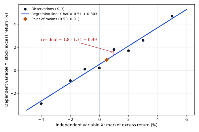
Worked example (data in the figure)
Eight monthly observations give , , and (both in %²). The underlying sums are and , and gives the same slope.
For the observation at with : , so the residual is .
Interpreting the coefficients
- Slope coefficient : how much the dependent variable is expected to move when the independent variable rises by one unit. In the example, a market excess return 1 percentage point higher goes with a stock excess return 0.80 point higher. When Y is a stock's excess return and X the market's, the slope is the stock's beta.
- Intercept : the predicted value of Y when X equals zero (where the line crosses the vertical axis).
- A large slope does not by itself mean a strong relationship; significance must be tested (t-test or confidence interval).
Types of data
Key concept
| Type | Definition | Example |
|---|---|---|
| Time series | Observations of one variable at regular intervals over time | A company's quarterly EPS for five years |
| Cross-sectional data | Observations of many subjects at one point in time | Today's closing prices of 30 stocks in an index |
| Panel data | Cross-sectional observations repeated over time | Quarterly EPS of 10 companies over five years |
Common exam traps
- The slope divides the covariance by the variance of X, the independent variable. Dividing by the variance of Y is a common error.
- OLS minimizes the squared differences between actual and predicted values of Y. It does not compare coefficients or X values.
- The slope is the change in Y per unit change in X. Reading it as the change in X per unit of Y reverses the roles.
Exam shortcuts
- The regression line passes through , so once the slope is known the intercept is with no further sums.
Bottom line
- Simple linear regression explains the variation of a dependent variable Y, , with the variation of a single independent variable X.
- Ordinary least squares chooses the line that minimizes the sum of squared errors, .
- The OLS estimates are and , so the fitted line passes through the point of means.
- The slope is the expected change in Y for a one-unit rise in X, and the intercept is the predicted value of Y when X equals zero.
- The residual is the gap between the actual and the fitted value; exam convention treats the residual, error term and disturbance term as the same thing, while current practice treats the residual as the sample estimate of the unobservable error term.
- Time series data follow one variable over time, cross-sectional data cover many subjects at one point in time, and panel data repeat cross-sectional observations over time.
Quick check
A credit analyst gathers data on 80 bond issuers at a single date to see whether an issuer's interest coverage ratio helps explain the yield spread on its bonds. In her simple linear regression, the dependent variable is:
Show answer and explanation
Correct answer: B
The dependent variable is the one whose variation the model explains, here the yield spread. The interest coverage ratio does the explaining, so it is the independent (explanatory) variable. Observations of many issuers at one date are cross-sectional data, which a simple linear regression can use as readily as time-series data.
Why the other options are wrong
- A. An explanatory variable is the independent variable. Making the coverage ratio the dependent variable reverses the roles set by the analyst's question.
- C. Data on many subjects at one point in time are cross-sectional data, and a regression can be run on them. Time-series data are not required.
Key takeaway Dependent variable (Y): explained, endogenous, predicted. Independent variable (X): explanatory, exogenous, predicting. The research question decides which is which.
Module 10.2
Analysis of Variance (ANOVA) and Goodness of Fit
LOS 10.b — Assumptions, residual analysis, ANOVA and goodness of fit
Assumptions of simple linear regression
Key concept
- Linearity: the relationship between X and Y is linear.
- Homoskedasticity: the residuals have the same variance for every observation.
- Independence: residuals are uncorrelated with one another (the X–Y pairs are independent).
- Normality: the residual term is normally distributed.
Violations show up in plots of the residuals against X (or against time). In a well-specified model the residuals scatter randomly around zero with no pattern.
| Violation | What the residual plot shows | Name |
|---|---|---|
| Nonlinear relationship | A systematic pattern, e.g., residuals positive, then negative, then positive as X rises | — |
| Residual variance not constant | Spread of residuals widens (or narrows) with X, or changes over time | Heteroskedasticity |
| Residuals correlated | Recurring pattern, e.g., large errors every December (seasonality); the estimated variances of the coefficients are then wrong | Autocorrelation |
| Residuals not normal | Skewed or fat-tailed residuals; hypothesis tests may be unreliable in small samples (with a large sample, the central limit theorem means the estimates may still be valid) | — |
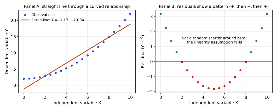
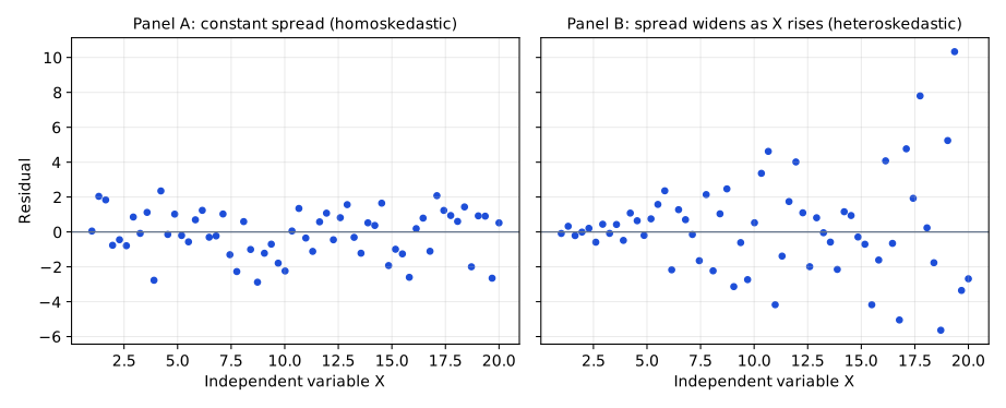
Outliers are observations far from the line. They can pull the estimated coefficients so that the line fits the other points poorly.
Analysis of variance (ANOVA)
Analysis of variance (ANOVA) splits the total variation of the dependent variable into an explained and an unexplained part:
- Total sum of squares (SST) : total variation.
- Sum of squares regression (SSR) : variation explained by the regression.
- Sum of squared errors (SSE) : unexplained variation (also called the residual sum of squares).
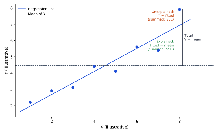
The sample variance of Y is its total variation divided by its degrees of freedom, .
- Mean square regression (MSR) ; with one independent variable (), MSR = SSR.
- Mean squared error (MSE) in a simple regression.
Key concept
| Source of variation | Degrees of freedom | Sum of squares | Mean sum of squares |
|---|---|---|---|
| Regression (explained) | SSR | MSR = SSR/1 | |
| Error (unexplained) | SSE | MSE = SSE/() | |
| Total | SST |
Goodness-of-fit measures
The standard error of estimate (SEE), also called the root mean squared error, is the standard deviation of the residuals; the lower it is, the better the fit.
Key concept
The coefficient of determination measures what fraction of the dependent variable's total variation the independent variable accounts for. In a simple regression , so the correlation coefficient is , with the sign of the slope. When only and SSR are known, SST SSR and SSE SST SSR, which then gives the MSE and the SEE.
F-test
The F-test compares the variation the regression explains, per degree of freedom, with the variation it leaves unexplained, per degree of freedom. A large ratio means the independent variable explains a lot relative to the noise.
The F-test asks whether the independent variables, as a group, explain the variation of Y; with several independent variables its null is that all slope coefficients are zero. With one independent variable, it tests vs. , the same hypothesis as the t-test of the slope. Reject if (a one-tailed test using the upper tail of the F-distribution). Rejecting means X and Y have a significant linear relationship.
Worked example
; SSR = 64 and SSE = 112, so SST = 176. MSE ; SEE ; ; (if the slope is positive); , well above the 5% critical value of about 4.2 for 1 and 28 degrees of freedom, so the slope is significant.
t-test of a regression coefficient
To test significance, set (two-tailed) and reject if . The test of the slope is equivalent to testing the correlation, . With one independent variable, the F-statistic equals the square of this t-statistic, so the F-test and the t-test of the slope always reach the same decision (in the worked example above, corresponds to ). The intercept can be tested the same way ().
Indicator variables
An indicator variable (dummy variable) takes the value 1 when a condition holds and 0 otherwise (e.g., 1 in recession quarters). Regressing Y on the indicator tests whether the condition matters: the slope equals the difference in the mean of Y between periods with and without the condition, and testing is equivalent to a difference-in-means test. The intercept is the mean of Y in periods without the condition (indicator = 0), and intercept plus slope is the mean in periods with it. Example. Regressing a company's quarterly earnings on a recession indicator tests whether earnings are cyclical; for cyclical earnings the slope is expected to be negative (lower earnings in recession quarters). If quarterly EPS averaged 1.40 in expansion quarters and 0.95 in recession quarters, the fitted line is , where in a recession quarter.
Common exam traps
- . SSE/SST is the unexplained share (), and SSR/SSE is not a standard measure. In the worked example, is the unexplained share; is 0.364.
- F is a ratio of mean squares, MSR/MSE. Dividing SSR by SSE ignores the degrees of freedom. In the worked example, instead of .
- SEE divides SSE by , the degrees of freedom, before taking the square root. Dividing by understates it. In the worked example, instead of 2.
- A negative slope gives a negative even though is positive. The standard error of the slope is a different statistic and is not a correlation.
Exam shortcuts
- With one independent variable, for the test of against , so at the same significance level the F-test and the two-tailed slope t-test reach the same decision and only one needs computing.
- When only and SSR are given, SST SSR and SSE SST SSR, which lead straight to the MSE and the SEE.
- In a simple regression , taking the sign of the slope.
Bottom line
- Simple linear regression assumes a linear relationship, homoskedastic residuals, residuals uncorrelated with one another, and normally distributed residuals.
- Residual variance that widens or narrows with X or over time is heteroskedasticity, and residuals correlated with one another, such as a recurring seasonal pattern, show autocorrelation.
- ANOVA splits total variation into explained and unexplained parts, .
- In a simple regression , , and , which equals .
- with 1 and degrees of freedom is a one-tailed test, and with one independent variable it tests , the same hypothesis as the slope's t-test.
- Regressing Y on an indicator variable gives a slope equal to the difference in the mean of Y between periods with and without the condition, and an intercept equal to the mean when the indicator is 0.
Quick check
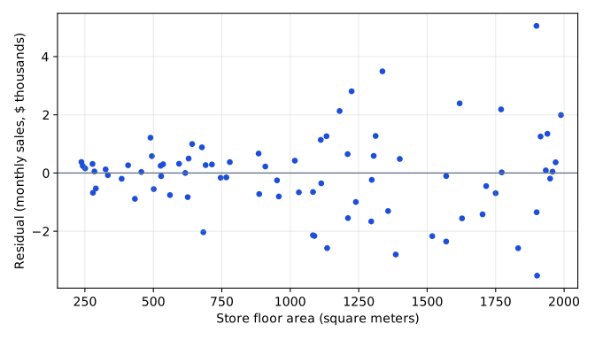
An analyst regresses the monthly sales of 80 stores on each store's floor area. The figure below plots the regression residuals against floor area. The pattern most likely indicates that the regression's residual term:
Show answer and explanation
Correct answer: A
The residuals fan out as floor area increases: their spread (variance) grows with the independent variable. A residual variance that is not constant across observations is heteroskedasticity, a violation of the homoskedasticity assumption.
Why the other options are wrong
- B. The plot shows residuals centered on zero with a changing spread; nothing in it points specifically to a nonnormal shape, and normality is judged from the shape of the residuals' distribution. How their spread changes with X is a separate question.
- C. Non-independence (autocorrelation) shows up as residuals that are correlated with one another, such as a recurring seasonal pattern over time. A widening spread with X is a variance problem.
Key takeaway Residual spread widening with X = heteroskedasticity (non-constant residual variance).
Module 10.3
Predicted Values and Functional Forms of Regression
LOS 10.c — Predicted values, prediction intervals and functional forms
Predicted values
A predicted value of the dependent variable plugs a forecast of the independent variable, , into the estimated equation:
Example: and : . Include the intercept and keep the sign of each term.
Confidence (prediction) interval for a predicted value
Key concept
where is the standard error of the forecast. At Level I it is usually given; if not:
Key concept
The forecast is more precise (smaller ) when the SEE is smaller, the sample is larger, is closer to , and the independent variable has a greater variance.
Example (continued): , , so and the two-tailed 5% critical value is 2.060. The 95% interval is , i.e., 1.71 to 7.89.
Computing when it is not given (a separate regression): SEE = 2.0, , , , :
The standard error of the forecast is always larger than the SEE: the forecast carries both the residual uncertainty and the uncertainty in the estimated coefficients.
| Interval | Centered on | Width driven by |
|---|---|---|
| Confidence interval for a coefficient | (or ) | Standard error of that coefficient |
| Prediction interval for Y | at | Standard error of the forecast |
Functional forms
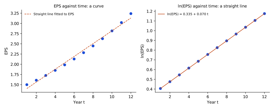
If the relationship between X and Y is not linear, taking natural logarithms of the dependent variable, the independent variable or both can make it linear. For example, EPS growing at a roughly constant percentage rate over time traces an upward curve.
Key concept
| Model | Equation | Slope interpretation | Typical use |
|---|---|---|---|
| Log-lin model | Relative (%) change in Y for an absolute change in X | Constant growth rate over time | |
| Lin-log model | Absolute change in Y for a relative (%) change in X | Y responds to proportional changes in X | |
| Log-log model | Relative change in Y for a relative change in X (an elasticity) | Both variables in proportional terms |
Example. In a log-lin regression of a company's annual EPS on a time index (1, 2, 3, …), a slope of 0.07 means EPS grows by roughly 7% a year (exactly ). It does not mean EPS rises by 0.07 currency units a year.
Choose the form by the nature of the variables and by comparing goodness-of-fit measures and residual plots.
- Exam convention: a higher , a higher F-statistic and a lower SEE indicate the better-fitting functional form.
- Current practice: and SEE are directly comparable only when the dependent variable is the same; a model of and a model of measure fit on different scales.
Common exam traps
- Prediction intervals use in a simple regression (two estimated parameters), not . In the example, 26 degrees of freedom give a critical value of 2.056 and an interval of 1.72 to 7.88 instead of 1.71 to 7.89.
- A prediction interval uses the standard error of the forecast . The standard error of the slope belongs to the interval for the slope coefficient.
- "Log" is attached to the variable that is logged: log-lin means Y is logged and X is linear.
Exam shortcuts
- The standard error of the forecast is always larger than the SEE, so a prediction interval narrower than SEE can be ruled out.
Bottom line
- A predicted value is , using the intercept and the sign of each term.
- The prediction interval for Y is with degrees of freedom, where is the standard error of the forecast.
- The forecast is more precise when the SEE is smaller, the sample is larger, is closer to and the independent variable has a greater variance.
- A log-lin model ( on X) has a slope giving the relative change in Y for an absolute change in X, a lin-log model the absolute change in Y for a relative change in X, and a log-log model an elasticity.
- Exam convention: a higher , a higher F-statistic and a lower SEE identify the better-fitting functional form; current practice: and SEE are directly comparable only when the dependent variable is the same.
Quick check
An analyst regresses a fertilizer producer's monthly stock returns on monthly changes in a crop price index, using 32 observations. The estimated coefficients are in the table below. She expects next month's change in the index to be −0.015 and computes a standard error of the forecast of 0.028. Critical t-values with 30 degrees of freedom are 1.310 with 10% in one tail and 1.697 with 5% in one tail. The 90% prediction interval for next month's return is closest to:
| Coefficient | Standard error | |
|---|---|---|
| Intercept | 0.0040 | 0.0035 |
| Crop price change | 0.6500 | 0.2100 |
Show answer and explanation
Correct answer: A
A prediction interval is the predicted value plus or minus the critical t-value times the standard error of the forecast. A two-sided 90% interval leaves 5% in each tail, so with n − 2 = 30 degrees of freedom the critical value is 1.697.
- Predicted return:
- Half-width:
- Interval: , that is, to
Calculator: 0.65 [×] 0.015 [=] gives 0.00975; 1.697 [×] 0.028 [=] gives 0.047516.
Why the other options are wrong
- B. This interval uses 1.310, the critical value with 10% in one tail. A two-sided 90% interval splits the 10% between the two tails, so each tail holds 5%.
- C. This interval is centered on , which drops the minus sign of the forecast change in the index.
Key takeaway Prediction interval , with n − 2 degrees of freedom and α/2 in each tail. Keep the sign of the forecast X when computing .
Module 10.4
Estimating CAPM Values With Simple Linear Regression
LOS 10.d — Estimating the CAPM with simple linear regression
The CAPM as a one-factor regression
The capital asset pricing model states
Because the only explanatory variable is the market risk premium, the CAPM is a one-factor risk model and can be estimated with simple linear regression, using past observations as proxies for expected values. Subtracting from both sides gives the estimable form:
Key concept
Key concept
| Regression element | CAPM meaning |
|---|---|
| Dependent variable | The asset's excess return |
| Independent variable | The market risk premium |
| Slope | The asset's estimated beta |
| Intercept | Return not explained by market exposure (zero if the CAPM holds exactly) |
Steps
- Collect data: the asset's returns; a security market index as the proxy for the market return; yields on short-term government debt as the proxy for the risk-free rate. At least 30 observations is the usual minimum (e.g., 1–3 years of weekly data or 3–5 years of monthly data).
- Compute the asset's excess returns and the market risk premium for each period.
- Run the least-squares regression of excess returns on the market risk premium.
- Use and an expected market risk premium to estimate the expected return: .
Testing and interpreting beta
Example: the slope is 1.25 with a standard error of 0.10 (large sample, so use z-values).
- Beta above 1: the stock's excess returns amplify the market's; below 1: they are dampened.
- Test : , so reject; beta is significantly different from zero.
- 95% confidence interval: to .
- Test (does the stock move one-for-one with the market?): , so reject; beta is significantly different from 1, and the estimate lies above it. This matches the interval above, which does not contain 1.
- A one-sided question, such as whether beta exceeds 1, uses versus , the same statistic and a one-tailed critical value.
- With and an expected market risk premium of 5%: .
Changing inputs: . With , a 0.4% rise in combined with a 0.4% fall in the market risk premium changes expected return by ; for a beta above 1 the same changes would lower it.
Reading a typical output
| Coefficient | Standard error | t-statistic | |
|---|---|---|---|
| Intercept | 0.05 | 0.08 | 0.63 |
| Market risk premium (slope) | 1.25 | 0.10 | 12.50 |
The slope row carries beta and its test; the intercept row is not significant here (t = 0.63), consistent with the CAPM's prediction of a zero intercept. The of such a regression tells how much of the asset's excess-return variation is systematic (market-driven); is the share that is unsystematic.
Choosing the sample
Longer samples give more observations and more precise estimates but risk including periods when the company's business mix, leverage and therefore beta were different. More frequent data (daily or weekly) add observations quickly but can be noisy for thinly traded assets. The choice depends on the purpose: a short-term speculator favors recent high-frequency data; a buy-and-hold investor favors monthly or quarterly data spanning at least one full business cycle.
Worked example: estimating and testing a CAPM beta
Sixty monthly observations of a stock's excess return and the market risk premium give a covariance of 0.00168 and a variance of the market risk premium of 0.00140. The regression reports a standard error of 0.16 for the slope, and with 60 observations the sample is large, so the two-tailed 5% critical value is 1.96. Estimate beta, test at the 5% level whether beta differs from 1, build the matching confidence interval for beta, and estimate the stock's expected return with a risk-free rate of 2.8% and an expected market risk premium of 5.5%.
Step 1. Beta is the slope coefficient: .
Step 2. Test against : . Because 1.25 is below 1.96, is not rejected, so beta is not significantly different from 1.
Step 3. The 95% confidence interval is , or 0.886 to 1.514. It contains 1, which agrees with Step 2.
Step 4. Expected return: .
Result. The estimated beta is 1.20, not significantly different from 1 at the 5% level, and the CAPM expected return is 9.4%.
Common exam traps
- The dependent variable is the asset's excess return and the independent variable is the market risk premium. A regression of raw returns on raw returns is not the CAPM specification.
- Beta is the slope coefficient. The intercept says nothing about beta, so a negative intercept does not make beta negative.
- Confidence interval for beta: slope critical value standard error of the slope. The intercept's standard error plays no part. With the output above, using the intercept's 0.08 gives 1.093 to 1.407 instead of 1.054 to 1.446.
Exam shortcuts
- A two-tailed 95% confidence interval for beta that excludes 1 means is rejected at the 5% level, and one that includes 1 means it is not, so either result gives the other.
Bottom line
- The CAPM is estimated by regressing the asset's excess return on the market risk premium ; the slope is the asset's beta and the intercept is zero if the CAPM holds exactly.
- A security market index proxies the market return, short-term government debt yields proxy the risk-free rate, and at least 30 observations is the usual minimum.
- Beta is tested with , and its confidence interval is the slope critical value the slope's standard error.
- The expected return is , and a change in inputs gives .
- The of the CAPM regression is the share of the asset's excess-return variation that is systematic, and is the unsystematic share.
- Longer samples give more precise estimates but may include periods with a different beta, and more frequent data can be noisy for thinly traded assets.
Quick check
To estimate a stock's beta, an analyst regresses the stock's excess returns on the market risk premium and obtains an intercept of −0.15 and a slope of 0.72. Based on this model, the stock's beta is:
Show answer and explanation
Correct answer: B
In the regression , the slope coefficient is the estimate of the asset's beta. The slope is 0.72, so beta lies between 0 and 1: the stock's excess returns tend to move less than one-for-one with the market risk premium.
Why the other options are wrong
- A. The negative number is the intercept, which is not beta. Beta is the slope, 0.72.
- C. A beta above 1 would require a slope above 1; the estimated slope is 0.72.
Key takeaway Beta = slope of the excess-return regression; the intercept is irrelevant to beta.
This reading has 29 questions in the full bank. Practice all of them.
Key Takeaways
- Dependent variable (Y): explained, endogenous, predicted. Independent variable (X): explanatory, exogenous, predicting. The research question decides which is which.
- Residual spread widening with X = heteroskedasticity (non-constant residual variance).
- Prediction interval , with n − 2 degrees of freedom and α/2 in each tail. Keep the sign of the forecast X when computing .
- Beta = slope of the excess-return regression; the intercept is irrelevant to beta.