Quantitative Methods · Reading 9

Simulation of Financial Asset Prices and Returns

CFA Level I · Quantitative Methods · Reading 9 · about 45 min

Quantitative Methods notes as a PDF166 pages · 2.6 MB · free, no sign-up · All PDFs

What you'll learn

LOS 9.a Describe historical simulation, its assumptions, strengths and weaknesses, and how it is used in investment applications such as VaR and bond portfolios.
LOS 9.b Describe bootstrap resampling (sampling with replacement), its strengths and weaknesses, and its investment applications.
LOS 9.c Describe Monte Carlo simulation, including multivariate simulation with the Cholesky decomposition, its strengths and weaknesses, and its investment applications.

Module 9.1

Historical Simulation

This reading describes three ways to simulate asset prices and returns: historical simulation, which applies actual past changes to current positions; bootstrap resampling, which draws from the observed sample with replacement; and Monte Carlo simulation, which draws from distributions the analyst specifies. For each method it covers the assumptions, investment applications such as VaR and option valuation, and the main strengths and weaknesses.

LOS 9.a — Historical simulation

What a simulation does

Key concept

A simulation is a predictive modeling technique that estimates the range of possible outcomes of a complex system (for example, a portfolio's return distribution, its risk, or future cash flows and liquidity) by running it through many scenarios. Every simulation follows the same four steps:

Set parameters: state the objective, choose the output variables, and define the calculations linking inputs to outputs.
Generate scenarios: create the input values for each trial (simple or drawn from complex distributions).
Evaluate scenarios: run each scenario through the calculation engine to produce outcome paths.
Compile and interpret results: aggregate the outcomes (e.g., into a distribution) and draw conclusions.

Historical simulation (this module), bootstrap resampling (Module 9.2) and Monte Carlo simulation (Module 9.3) differ mainly in step 2, where the scenarios come from.

Historical simulation

Historical simulation applies actual past changes in prices, returns or risk factors to the current portfolio positions. It assumes that past data represent the future (past performance is a reliable guide to future outcomes and risks, and the historical record stands in for the population of outcomes). When the parameters are set, the chosen dates and risk factors may need simplifying assumptions so that all returns cover the same time frame. Equity inputs are usually logarithmic (continuously compounded) price returns, and percentage returns work as well; for bonds, the simulated yields serve as discount rates for the future cash flows.

Key concept

Strengths	Weaknesses
Easy to explain — narratives are built around real past events	Assumes the past repeats; weak when there are regime changes or unprecedented events
Nonparametric — no need to force the data into a distribution such as the normal; handles excess kurtosis, skewness and fat tails, and captures extreme events and drift better than a parametric model	Can only produce outcomes that actually occurred in the lookback period
Captures volatility clustering (calm and turbulent periods tend to persist)	Results depend on the quality and completeness of the data

Missing data and proxies

Gaps in the historical record arise from thinly traded instruments, asynchronous global markets (holidays, outages, trading halts), and securities that did not exist during part of the period (e.g., a recent IPO). The fix is a proxy: a substitute instrument, or a weighted combination of instruments with data available, that stands in for the missing observations.

Application: value at risk (VaR)

Key concept

Value at risk (VaR) is the minimum loss expected over a specified period in the worst 5% (or 1%) of outcomes. Equivalently, it is the maximum potential loss at the matching level of confidence (95% or 99%); larger losses still occur in the tail. Using historical simulation for a long-only portfolio:

Set parameters: compute daily (usually logarithmic) returns of each asset over the lookback period.
Generate scenarios: apply each day's returns to today's positions to get one profit-or-loss (P&L) figure per historical day.
Evaluate scenarios: build the P&L distribution (e.g., a histogram).
Compile and interpret: rank the P&L from worst to best; the 95% VaR is the fifth percentile of the distribution. If the percentile falls between two observations, use either neighbor or a weighted average.

Example (historical vs. parametric VaR). A $4 million equity portfolio is revalued under each of the last 500 daily return scenarios. Five percent of 500 is 25 outcomes, so the fifth percentile lies between the 25th-worst P&L (−$118,000) and the 26th-worst (−$114,000). The 1-day 95% historical VaR is therefore about $116,000 (the average of the two neighbors; either neighbor is also acceptable). A parametric VaR that assumes normal returns, a zero daily mean and a daily standard deviation of 1.5% gives $1.645 \times 0.015 \times $4, 000, 000 = $98, 700$ . The historical figure is larger because the actual return distribution has a fatter left tail than the normal distribution allows.

Because VaR focuses on the loss tail, a few large gains barely affect it. For daily VaR, analysts usually assume a mean return of zero, because a daily drift is hard to distinguish statistically from zero (the null hypothesis of no directional move) and daily volatility dwarfs any trend.

Application: bonds

A bond's historical prices are misleading because its interest-rate sensitivity (duration) shrinks as it approaches maturity: a 10-year zero-coupon bond bought five years ago now behaves like a 5-year bond. Historical simulation for bonds therefore uses historical changes in yields (for example, benchmark yields for the same remaining maturity) and applies them to today's cash flows. To simulate a bond with three years to maturity, use yield changes that were observed on bonds that had three years left to maturity at the time.

Common exam traps

Historical simulation assumes past data represent the future. Fitting a statistical model to the population describes Monte Carlo simulation, and resampling with replacement describes bootstrapping.
Historical 95% VaR is the fifth percentile of the simulated P&L distribution (about the 25th-worst of 500 outcomes) rather than the single worst outcome.
A proxy fills missing data; it is not a risk factor or a hypothetical scenario.

Exam shortcuts

With $N$ historical scenarios, the 95% VaR lies between the $(0.05 N)$ th-worst P&L and the next-worst one, so only those two outcomes need to be located (either one or a weighted average of the two is acceptable).

Bottom line

Every simulation sets parameters, generates scenarios, evaluates them and compiles the results; historical simulation, bootstrapping and Monte Carlo simulation differ mainly in where the scenarios come from.
Historical simulation applies actual past changes in prices, returns or risk factors to the current portfolio positions and assumes that past data represent the future.
Historical simulation is nonparametric and captures skewness, excess kurtosis, fat tails and volatility clustering, but it can only produce outcomes from the lookback period and is weak when there are regime changes or unprecedented events.
Missing historical data are filled with a proxy, a substitute instrument or a weighted combination of instruments with data available.
VaR is the minimum loss over a specified period in the worst 5% (or 1%) of outcomes; the 95% historical VaR is the fifth percentile of the simulated P&L distribution, and daily VaR usually assumes a mean return of zero.
Because a bond's duration shrinks as it approaches maturity, historical simulation for bonds applies past yield changes for the same remaining maturity to today's cash flows instead of using the bond's own past prices.

Quick check

Question 1Core

Which of the following is most likely an advantage of historical simulation compared with a parametric approach that assumes normally distributed returns?

Show answer and explanation

Correct answer: B

Historical simulation is nonparametric: it uses actual past changes, so the scenarios automatically carry the fat tails, skewness and volatility clustering present in the data. A normal-distribution model tends to understate extreme outcomes.

Why the other options are wrong

A. Reliance on the past is the main weakness of historical simulation; after a regime change, past data may no longer represent the future.
C. Historical simulation can only reproduce outcomes that actually occurred in the lookback period; simulating conditions never seen before is an advantage of Monte Carlo simulation.

Key takeaway Historical simulation is nonparametric, captures fat tails and volatility clustering and is easy to explain; its limit is that it can only replay what actually happened.

Module 9.2

Bootstrap Resampling

LOS 9.b — Bootstrap resampling

How bootstrapping works

Key concept

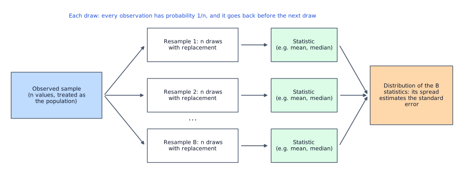
Bootstrap resampling (bootstrapping) is a nonparametric simulation method. It treats the observed historical sample as a proxy for the population and creates many new datasets by drawing observations from it at random with replacement: each observation is drawn, used, and put back so that it can be drawn again. Drawing a random value in this way is called pulling.

With a dataset of $n$ observations, each observation has a probability of $1/ n$ of being selected on every draw.
Within one scenario, the same observation can be drawn as many times as there are draws in that scenario.
Across scenarios, the same observation can appear in many samples (or in none).

Example. To simulate a 6-month path from 60 historical monthly returns, draw six random integers from 1 to 60 and look up the corresponding returns. Any single month has a 1/60 chance on each draw and could, in principle, appear up to six times in the same path (though that is very unlikely). Repeat thousands of times.

Flow diagram: an observed sample of n values, treated as the population, feeds resamples 1, 2 to B, each of n draws with replacement (every observation has probability 1/n on each draw). Each resample gives a statistic such as a mean or median, and the distribution of the B statistics gives the standard error. — How bootstrap resampling builds a sampling distribution

Bootstrapping vs. historical simulation

The two methods treat the data differently. Historical simulation replays the past dataset directly, as if it were the population, so each scenario is a sequence of events that actually happened. Bootstrapping treats the observed sample as a proxy for the population and builds new combinations of past observations by resampling with replacement. Module 9.3 compares all three simulation methods side by side.

Bootstrapping needs no theoretical model. Each resample gives one value of the statistic of interest (a mean, say), so thousands of resamples trace out an approximate sampling distribution of that statistic even when the original dataset is small. The spread of that distribution makes the stability of an estimate easy to assess. The repeated resampling takes somewhat more computation than historical simulation. Because it preserves the empirical distribution of the data while reshuffling it, it reduces the risk of overfitting to one particular historical sequence. It suits finance problems in which the population distribution is unknown but can be inferred from the sample.

Applications

European-style call option values at maturity. A European call can be exercised only at maturity and is valuable only if the underlying price ends above the exercise price, so the objective is the option's value at maturity. Resample historical returns to build many price paths over the investment period, compute the option payoff at the end of each path, and study the resulting distribution and its mean. This avoids the constant-volatility and normality assumptions of theoretical option-pricing models. Because of the option's leverage and limited downside, the distribution of option values can be more skewed than the distribution of share prices. The result is the distribution of terminal payoffs under historical (real-world) returns. It is not by itself the option's current no-arbitrage price: discounting a real-world average payoff at the risk-free rate would not give that price (Module 9.3 sets out the conditions for Monte Carlo pricing).
Estimating the volatility of target date funds (which shift toward less risky assets as the retirement date approaches): bootstrap monthly returns, compute the standard deviation of each simulated series, and compare ranges across funds to judge which is more aggressive.

Strengths and weaknesses

Key concept

Strengths	Weaknesses
Minimal assumptions — no need to specify a distribution such as the normal	Sensitive to sample quality — any bias in the original sample is carried into every resample
Simple to implement	Computationally intensive for thousands of resamples on large datasets
Statistically robust — reliable estimates of the variability of a statistic, even from small samples	No analytical insight — estimates, but no theoretical explanation
Reliable standard errors and confidence intervals, less influenced by outliers	Limited extrapolation — cannot generate outcomes outside the range of observed data (weak for extreme tail events)
Adaptable to many statistics (mean, median, correlation)	Not suited to autocorrelated time series — random resampling breaks the time-sequence dependence
Works with the sample at hand; no large external datasets needed

Bootstrapping is useful when the data show time-varying volatility, skewness or fat tails that are hard to model parametrically, and when historical patterns are expected to persist. It complements analytic methods, which explain the underlying relationships in more detail.

Common exam traps

Bootstrapping makes no distributional assumption; Monte Carlo is the method that requires one.

Bottom line

Bootstrapping is a nonparametric method that uses the sample at hand as a proxy for the population and builds new datasets by drawing from it at random with replacement, so each of $n$ observations has a $1/ n$ chance on every draw.
In bootstrapping the same observation can be drawn several times within one scenario and can appear in many samples or in none.
Historical simulation replays the past dataset as if it were the population, while bootstrapping builds new combinations of past observations, which reduces the risk of overfitting to one historical sequence.
Bootstrapping can give the distribution of a European call's payoff at maturity under historical returns, which is not by itself the option's current no-arbitrage price, and can estimate the volatility of target date funds.
Bootstrapping needs minimal assumptions and works with small samples, but it carries any bias in the original sample into every resample, cannot generate outcomes outside the observed range and is not suited to autocorrelated time series.

Quick check

Question 2Core

An analyst builds each bootstrap scenario for an eight-quarter horizon by drawing from a dataset of 40 historical quarterly returns. Within a single scenario, any one historical observation can be drawn:

Show answer and explanation

Correct answer: A

Bootstrapping samples with replacement: after each draw the observation is returned to the dataset. An eight-quarter scenario needs eight draws, so the same observation could in principle be pulled on every one of them, although with a 1/40 chance per draw this is extremely unlikely.

Each scenario consists of 8 draws of a random integer from 1 to 40, each mapped to one historical quarterly return. The probability that a given observation is chosen on any single draw is $1/40$ , and the maximum number of appearances in one scenario equals the number of draws, 8.

Why the other options are wrong

B. "Only once" describes sampling without replacement. Bootstrap resampling replaces each observation, so repeats are possible.
C. Forty is the size of the dataset; a scenario of eight quarters contains only eight draws.

Key takeaway Sampling with replacement: repeats are possible, capped by the number of draws in the scenario.

Module 9.3

Monte Carlo Simulation

LOS 9.c — Monte Carlo simulation

The method

Monte Carlo simulation generates scenarios by random sampling from probability distributions specified by the analyst (normal, lognormal, or any other shape with any parameters) rather than from raw historical observations. Running thousands of trials produces a simulated frequency distribution of prices or returns, from which risk and performance measures are estimated. The analyst should run as many trials as practical: more trials give more precise estimates, and the number of trials is limited essentially by computational power and time. Because the analyst controls the input assumptions, the sensitivity of the output to each assumption can be tested ("what if" analysis).

Applications

Portfolio performance over a future horizon: expected return and standard deviation to a chosen level of confidence.
Valuing securities without an analytic (closed-form) pricing formula, such as path-dependent options (e.g., Asian-style options, whose payoff depends on an average price), mortgage-backed securities (the borrowers' prepayment option acts like an embedded call) and convertible bonds.
European call options.
- Exam convention: a Monte Carlo value for a European call should match the Black-Scholes-Merton value, and it gets closer as more trials are run.
- Current practice: this holds only when the simulated price dynamics match the Black-Scholes-Merton assumptions: a lognormal price with constant volatility and, for pricing, an expected return equal to the risk-free rate less any dividend yield (risk-neutral valuation). The average payoff discounted at the risk-free rate then converges to the Black-Scholes-Merton value as the number of trials grows. A lognormal assumption alone is not enough: simulating with a real-world expected return and then discounting at the risk-free rate would not reproduce that value.

Steps for an option: (1) set the horizon, risk-free rate, the price distribution (e.g., lognormal), volatility and expected return; (2) draw random numbers to create price paths; (3) compute the payoff on each path over thousands of trials; (4) average the payoffs and discount at the risk-free rate.

Multivariate simulation and the Cholesky decomposition

When several variables move together (a portfolio, or an option on several assets), the simulated inputs must have the right correlation. Under the usual lognormal price model, the assets' log returns are assumed to be jointly normal, and the inputs are each asset's volatility and the correlations between returns. The Cholesky decomposition factorizes the covariance (or correlation) matrix and maps independent standard normal draws into correlated normal variables, which are then used to generate the simulated paths. For two variables with independent draws $Z_{1}$ and $Z_{2}$ (mean 0, standard deviation 1):

Key concept

X_{1} = σ_{1} Z_{1}, X_{2} = σ_{2} (ρ Z_{1} + 1 - ρ^{2} Z_{2})

Example. With $σ_{1} = 10%$ , $σ_{2} = 15%$ , $ρ = 0.8$ and draws $Z_{1} = 0.5$ and $Z_{2} = 1.0$ , $X_{1} = 5%$ ; $X_{2} = 15% (0.8 \times 0.5 + 0.6 \times 1.0) = 15%$ .

Strengths and weaknesses

Key concept

Strengths	Weaknesses
Wide applicability — assets, risk factors, portfolios; nonlinear relationships, time-varying volatility, fat tails	Complexity — needs modeling expertise and a time-consuming set-up
Flexibility for nonnormal distributions (skewness, excess kurtosis)	Model dependency — results are only as good as the assumed distributions and parameters
Precision given enough trials	Computational intensity — slow and costly for real-time use
Correlation handling among many assets	Data requirements — extensive data to estimate parameters such as volatilities and correlations
Forward-looking — can simulate hypothetical or extreme conditions never seen in history	Gives a statistical estimate, not an exact answer, and cannot provide the cause-and-effect insight of analytic methods

Monte Carlo is usually run alongside analytic methods. Where no analytic method can be applied, it can serve as the valuation tool itself, and its robustness is checked by changing the assumptions and rerunning.

Comparing the three methods

Key concept

Feature	Historical simulation	Bootstrapping	Monte Carlo simulation
Data source	Historical dataset	Observed sample	Assumed (modeled) distribution
Sampling	Directly from history	Resampling with replacement	Random draws from a specified distribution
Assumption	Past data represent the future	Sample represents the population	Process generating outcomes can be modeled statistically
Typical uses	Risk management, stress tests	Confidence intervals, standard errors	Complex systems, long-term outcomes
Flexibility	Limited to historical patterns	Limited by sample size	Highly flexible, hypothetical scenarios
Uncertainty captured	Only what was observed in history	Variability from resampling	Hypothetical uncertainty from the modeled inputs
Computational intensity	Low to moderate	Moderate	High

Common exam traps

The Cholesky decomposition generates correlated paths from an assumed correlation; it does not estimate correlations or covariances.

Exam shortcuts

Identify the method from the source of the scenarios: actual past changes mean historical simulation, resampling with replacement from the observed sample means bootstrapping, and random draws from an assumed distribution mean Monte Carlo simulation.

Bottom line

Monte Carlo simulation draws scenarios from probability distributions specified by the analyst and runs thousands of trials to build a simulated frequency distribution, with more trials giving more precise estimates.
Monte Carlo simulation is used to estimate portfolio performance and to value securities without a closed-form pricing formula, such as Asian-style options, mortgage-backed securities and convertible bonds.
Exam convention: a Monte Carlo value for a European call should match the Black-Scholes-Merton value, getting closer as more trials are run; current practice: this holds only when the simulated prices are lognormal with constant volatility and a risk-neutral expected return, with the average payoff discounted at the risk-free rate.
The Cholesky decomposition maps independent standard normal draws into correlated normal variables using an assumed correlation; it does not estimate correlations or covariances.
Monte Carlo simulation is flexible, forward-looking and handles nonnormal distributions and correlations, but it is complex, model-dependent, computationally intensive and data-hungry, and it gives a statistical estimate without the cause-and-effect insight of analytic methods.
Historical simulation assumes past data represent the future, bootstrapping assumes the sample represents the population, and Monte Carlo simulation assumes the process generating outcomes can be modeled statistically.

Quick check

Question 3Core

Compared with historical simulation and bootstrap resampling, an advantage of Monte Carlo simulation is that it:

Show answer and explanation

Correct answer: C

Monte Carlo scenarios are generated from distributions chosen by the analyst, so the method can simulate hypothetical or extreme conditions that never appeared in the historical record. Historical simulation and bootstrapping can only reuse what actually happened.

Why the other options are wrong

A. Monte Carlo usually has heavy data requirements, because volatilities, correlations and other parameters must be estimated.
B. Monte Carlo models are more complex and harder to communicate than methods that replay or resample actual history.

Key takeaway Monte Carlo is forward-looking: it can model scenarios with no historical precedent.

This reading has 16 questions in the full bank. Practice all of them.

Key Takeaways

Historical simulation is nonparametric, captures fat tails and volatility clustering and is easy to explain; its limit is that it can only replay what actually happened.
Sampling with replacement: repeats are possible, capped by the number of draws in the scenario.
Monte Carlo is forward-looking: it can model scenarios with no historical precedent.