Quantitative Methods · Reading 8

Portfolio Standard Deviation

CFA Level I · Quantitative Methods · Reading 8: The Return and Risk of a Financial Portfolio · about 1 h 28 min

Quantitative Methods notes as a PDF166 pages · 2.6 MB · free, no sign-up · All PDFs

What you'll learn

LOS 8.a Calculate and interpret the expected return, variance, standard deviation, covariance and correlation of portfolio returns, including multiperiod returns and the effects of portfolio drift and diversification.
LOS 8.b Describe, calculate and interpret the minimum-variance portfolio, the efficient frontier and portfolios that combine a risky portfolio with the risk-free asset.
LOS 8.c Explain optimal portfolio selection given an investor's risk aversion and the capital allocation line, the extension to the market portfolio and the capital market line, and the CAPM.

Module 8.1

Portfolio Expected Return

This reading computes a portfolio's expected return, variance and standard deviation from its weights, standard deviations and covariances or correlations, and shows how lower correlation produces a diversification benefit. It then derives the minimum-variance portfolio and the efficient frontier, combines a risky portfolio with a risk-free asset along the capital allocation line, selects an optimal portfolio from an investor's risk aversion and indifference curves, and extends the analysis to the capital market line, beta and the CAPM.

LOS 8.a — Portfolio expected return, historical returns and portfolio drift

Why portfolio statistics matter

Managing a portfolio means working with a small set of statistics: the expected returns, standard deviations and correlations of the holdings. These can be historical (built from realized past returns) or forward-looking (built from forecasts or models). Historical data are a sensible anchor, but a short history can give biased estimates; forecasts can blend history with economic views. Either way, the estimates must be revisited regularly.

Expected return of a portfolio

The expected return of a portfolio is the weighted average of the expected returns of its assets, where each weight is the asset's share of total portfolio value:

Key concept

E (R_{P}) = i = 1 \sum N w_{i} E (R_{i}), i = 1 \sum N w_{i} = 1

Example. A portfolio holds 30% in a fund expected to earn 5% and 70% in a fund expected to earn 9%, so $E (R_{P}) = 0.30 (5%) + 0.70 (9%) = 7.8%$ .

The historical return of a portfolio for one period is the same weighted average applied to realized returns:

R_{P, t} = i = 1 \sum N w_{i, t - 1} R_{i, t}

where $w_{i, t - 1}$ is the weight at the start of period $t$ .

Multiperiod returns: arithmetic vs. geometric

Key concept

Measure	Formula	Comment
Sum of period returns (cumulative arithmetic return)	$\sum_{t = 1}^{T} R_{P, t}$	Adds the period returns; ignores compounding
Arithmetic average	$R ˉ_{P} = \frac{1}{T} \sum_{t = 1}^{T} R_{P, t}$	Ignores compounding
Cumulative (compound) return	$R_{P, T} = \prod_{t = 1}^{T} (1 + R_{P, t}) - 1$	Assumes income is reinvested and no capital is added or withdrawn
Geometric average	$R ˉ_{g, P} = [\prod_{t = 1}^{T} (1 + R_{P, t})]^{1/ T} - 1$	Compound growth rate per period

If the portfolio is not rebalanced, the cumulative return over the whole period equals the weighted average of each asset's cumulative return using the initial weights: $R_{P, T} = \sum_{i} w_{i, 0} [\prod_{t = 1}^{T} (1 + R_{i, t}) - 1]$ . With or without drift, the formulas in the table are applied to the period-by-period portfolio returns $R_{P, t}$ .

Portfolio drift and style drift

Market moves change the weights: winners grow and losers shrink. This is portfolio drift. With no rebalancing, each period's return must be computed with the new (drifted) weights, which come from the start-of-period market values.

Style drift is a portfolio moving away from its stated strategy. It can come from portfolio drift (a strong equity market pushes a balanced portfolio overweight in stocks) or from changes in the holdings themselves (a small-cap stock that grows into the mid-cap category). Portfolio drift can sometimes offset style drift, but managers still monitor and rebalance to keep a portfolio aligned with its goals.

Key concept

How drift changes a portfolio depends on the starting weights.

Exam convention: in an equal-weighted portfolio, drift raises the weights of the high-return securities, so performance tilts toward higher-growth or higher-volatility assets; in a portfolio that is not equally weighted, drift tends to enlarge the already large allocations, so the portfolio behaves like a momentum strategy and its concentration risk may rise.
Current practice: in any unrebalanced portfolio, whichever assets outperform gain weight and underperformers lose weight. Whether concentration or overall risk rises depends on which assets outperform: if the largest positions (or the more volatile assets) do best, concentration and risk increase; if smaller positions outperform, the weights can move closer together (e.g., an 80/20 portfolio whose assets return 0% and 100% drifts to about 67/33). A high realized return does not by itself mean the asset is high-volatility.

Worked example — returns with changing weights

A client invests $50,000 in Asset A and $50,000 in Asset B and never rebalances. Returns: A earns 10% in Period 1 and −4% in Period 2; B earns 2% and then 8%.

Period 1 return $= 0.50 (10%) + 0.50 (2%) = 6.00%$ . End values: A = $55,000, B = $51,000 (total $106,000).
New weights: A $= 55, 000/106, 000 = 51.89%$ ; B $= 48.11%$ .
Period 2 return $= 0.5189 (- 4%) + 0.4811 (8%) = 1.77%$ .
Cumulative return $= (1.06) (1.0177) - 1 = 7.88%$ (check: end value $52,800 + $55,080 = $107,880). Arithmetic average $= (6.00% + 1.77%) /2 = 3.89%$ ; the simple sum of the two period returns is 7.77%, below the compound 7.88%.

Common exam traps

Expected return is a weighted average of expected returns only; do not plug in variances or correlations.
Applying the original weights to a later period of an unrebalanced portfolio gives the wrong return: 2.00% instead of 1.77% for Period 2 in the example.
A holding that grows from small cap into the mid-cap category causes style drift; portfolio drift refers only to weights shifting with market values.

Exam shortcuts

For a portfolio that is not rebalanced, the cumulative return equals the initial-weight average of each asset's cumulative return, so the cumulative figure needs no period-by-period weights.

Bottom line

A portfolio's expected return is the weighted average $E (R_{P}) = \sum w_{i} E (R_{i})$ , with each weight equal to the asset's share of total portfolio value and the weights summing to 1.
A portfolio's historical return for one period is $\sum w_{i, t - 1} R_{i, t}$ , using the weights at the start of the period.
The cumulative (compound) return $\prod (1 + R_{P, t}) - 1$ and the geometric average include compounding, while the sum and the arithmetic average of the period returns ignore it.
Without rebalancing, market moves shift the weights (portfolio drift), so each period's return must use the drifted weights from start-of-period market values.
Style drift is a portfolio moving away from its stated strategy, either through portfolio drift or through changes in the holdings themselves, such as a small-cap stock growing into the mid-cap category.
Exam convention: drift raises the weights of high-return securities in an equal-weighted portfolio and enlarges already large allocations in a portfolio that is not equally weighted, so it behaves like a momentum strategy with possibly higher concentration risk; current practice: in any unrebalanced portfolio the outperformers gain weight, and whether concentration or risk rises depends on which assets outperform.

Quick check

Question 1Core

Nadia Okafor builds the two-fund portfolio shown in the table below and does not rebalance it at any point. Okafor's portfolio return for Year 2 is closest to:

Okafor portfolio: starting values and annual returns

Holding	Value at start of Year 1	Return in Year 1	Return in Year 2
Equity fund	$60,000	20%	−10%
Bond fund	$40,000	2%	6%

Show answer and explanation

Correct answer: C

Without rebalancing, the weights drift with market values (portfolio drift). Each period's portfolio return must use the weights at the start of that period, so the Year 2 return is computed with the weights at the end of Year 1, not the original 60/40 split.

1. Values at the end of Year 1

Equity fund: $$60, 000 \times 1.20 = $72, 000$ ; bond fund: $$40, 000 \times 1.02 = $40, 800$ ; total $= $112, 800$ .

2. Weights at the start of Year 2

w_{equity} = \frac{72 , 000}{112 , 800} = 0.6383, w_{bond} = \frac{40 , 800}{112 , 800} = 0.3617

3. Year 2 portfolio return

R_{P, 2} = 0.6383 (- 10%) + 0.3617 (6%) = - 6.383% + 2.170% = - 4.21%

Check: end values $$64, 800 + $43, 248 = $108, 048$ ; $108, 048/112, 800 - 1 = - 4.21%$ .

Why the other options are wrong

A. −2.00% is the equal-weighted average of the two Year 2 returns, $(- 10% + 6%) /2$ ; it ignores both the original and the drifted weights.
B. −3.60% uses the original weights, $0.60 (- 10%) + 0.40 (6%)$ . That would be right only if the portfolio had been rebalanced back to 60/40 at the end of Year 1.

Key takeaway No rebalancing means the weights drift: recompute each weight from start-of-period market values before weighting the period's returns.

Module 8.2

Portfolio Risk Measures

LOS 8.a — Variance and standard deviation of a portfolio

Portfolio variance

Risk is measured by how far returns scatter around their mean: the variance and its square root, the standard deviation. Because the standard deviation is in the same units as returns, it is the usual headline risk number.

For $N$ assets, portfolio variance depends on the weights, each asset's variance and every pair's covariance:

σ_{P}^{2} = i = 1 \sum N j = 1 \sum N w_{i} w_{j} Cov (R_{i}, R_{j})

For two assets the formula becomes:

Key concept

σ_{P}^{2} = w_{1}^{2} σ_{1}^{2} + w_{2}^{2} σ_{2}^{2} + 2 w_{1} w_{2} Cov_{1, 2}

σ_{P} = σ_{P}^{2}

Covariance and correlation

Covariance is often given indirectly through the correlation (correlation coefficient) $ρ_{1, 2}$ , which is bounded between −1 and +1:

Key concept

Cov_{1, 2} = ρ_{1, 2} σ_{1} σ_{2} ⟹ σ_{P}^{2} = w_{1}^{2} σ_{1}^{2} + w_{2}^{2} σ_{2}^{2} + 2 w_{1} w_{2} ρ_{1, 2} σ_{1} σ_{2}

For forward-looking (expected) values the identity does not hold mechanically, because joint variability and nonlinear interactions among the three inputs also matter. Exam calculations use the identity above.

Special cases

Key concept

Correlation	Portfolio standard deviation (two assets, positive weights)	Diversification benefit
$ρ = + 1$	$σ_{P} = w_{1} σ_{1} + w_{2} σ_{2}$ (weighted average)	None
$- 1 < ρ < + 1$	Below the weighted average	Some; larger as $ρ$ falls
$ρ = - 1$	$σ_{P} = ∣ w_{1} σ_{1} - w_{2} σ_{2} ∣$	Maximum; zero risk only when $w_{1} σ_{1} = w_{2} σ_{2}$

Worked example

A portfolio is 20% in Asset J (standard deviation 25%) and 80% in Asset K (standard deviation 10%); the correlation is 0.20.

σ_{P}^{2} = (0.20)^{2} (0.25)^{2} + (0.80)^{2} (0.10)^{2} + 2 (0.20) (0.80) (0.20) (0.25) (0.10)

= 0.0025 + 0.0064 + 0.0016 = 0.0105 σ_{P} = 0.0105 = 10.25%

The weighted average of the two standard deviations is $0.20 (25%) + 0.80 (10%) = 13%$ ; the gap (13% vs. 10.25%) is the diversification benefit.

Worked example — covariance given directly, three-asset extension

If the covariance is given, use it as is. Two assets with $σ_{1}^{2} = 0.0400$ , $σ_{2}^{2} = 0.0225$ and $Cov_{1, 2} = - 0.0030$ , held 60/40:

σ_{P}^{2} = 0.36 (0.0400) + 0.16 (0.0225) + 2 (0.60) (0.40) (- 0.0030) = 0.0144 + 0.0036 - 0.00144 = 0.01656, σ_{P} = 12.87%

The negative covariance makes the third term negative, so the portfolio is far less risky than a 60/40 average of the standard deviations ( $0.6 \times 20% + 0.4 \times 15% = 18%$ ) would suggest. With three assets, the variance has three weighted-variance terms and three covariance terms, each doubled:

σ_{P}^{2} = i = 1 \sum 3 w_{i}^{2} σ_{i}^{2} + 2 w_{1} w_{2} Cov_{1, 2} + 2 w_{1} w_{3} Cov_{1, 3} + 2 w_{2} w_{3} Cov_{2, 3}

Calculator tip

Compute each of the three terms separately, add them, then take the square root last. Keep returns in decimals throughout (0.25 rather than 25) or in percent throughout; mixing the two gives wrong answers.

Common exam traps

Forgetting the factor 2 in the covariance term. In the J/K example, this gives $0.0097 = 9.85%$ instead of 10.25%.
Using variances instead of standard deviations inside $ρ σ_{1} σ_{2}$ . In the J/K example, $0.20 \times 0.0625 \times 0.0100$ as the covariance gives a variance of 0.00894 and a standard deviation of 9.46%, instead of 10.25%.
Reporting the variance as if it were the standard deviation (e.g., 0.0105 read as "1.05%").
Averaging the standard deviations when $ρ < 1$ : that is correct only for perfect positive correlation. In the J/K example, this gives 13% instead of 10.25%.
Assuming $ρ = - 1$ always means zero risk: it does only at one specific set of weights.

Exam shortcuts

For two assets with positive weights, the portfolio standard deviation equals the weighted average of the two standard deviations only when $ρ = + 1$ and is below it for any lower correlation, so with $ρ < + 1$ an answer at or above the weighted average can be ruled out.

Bottom line

Two-asset portfolio variance is $σ_{P}^{2} = w_{1}^{2} σ_{1}^{2} + w_{2}^{2} σ_{2}^{2} + 2 w_{1} w_{2} Cov_{1, 2}$ , and the portfolio standard deviation is its square root.
Covariance can be written $Cov_{1, 2} = ρ_{1, 2} σ_{1} σ_{2}$ , which exam calculations use, although for forward-looking expected values the identity does not hold mechanically.
With positive weights, a correlation of +1 gives a portfolio standard deviation equal to the weighted average of the standard deviations (no diversification benefit), and any lower correlation gives less, with a larger benefit as $ρ$ falls.
With $ρ = - 1$ , $σ_{P} = ∣ w_{1} σ_{1} - w_{2} σ_{2} ∣$ , which is zero only when $w_{1} σ_{1} = w_{2} σ_{2}$ .
A negative covariance makes the cross term negative, so the portfolio is much less risky than the weighted average of the standard deviations suggests.

Module 8.3

Correlation and Diversification Benefits

LOS 8.a — Correlation, diversification and portfolios of many assets

Correlation drives the diversification benefit

Changing the weights of two assets traces out a curve of attainable risk–return combinations. When the assets are less than perfectly correlated, the curve bows to the left: moving from the riskier asset toward the safer one cuts risk faster than it cuts return. This is the diversification benefit, and it grows as correlation falls. At $ρ = + 1$ the combinations lie on a straight line; at $ρ = - 1$ one mix has zero risk.

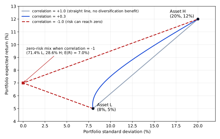
Risk-return curves for mixes of Asset L (standard deviation 8%, expected return 5%) and Asset H (standard deviation 20%, expected return 12%). With correlation +1.0 the mixes lie on a straight line between the two assets (no diversification benefit). With correlation +0.3 the curve bows to the left of that line. With correlation -1.0 the mixes form two straight segments meeting at zero risk: the zero-risk mix is 71.4% in L and 28.6% in H with an expected return of 7.0%. — Two-asset portfolios under different return correlations

Of all the feasible mixes, the efficient ones are those with the highest return for their level of risk, which lie on the upper part of the curve.

More assets: the variance–covariance matrix

With $N$ assets, the variance-covariance matrix has $N$ variances on its diagonal and

Key concept

number of unique covariances = \frac{N ^{2} - N}{2}

So 20 assets require $(400 - 20) /2 = 190$ covariances. Normalizing the covariance matrix gives a correlation matrix, which helps an investor spot the pairs with the lowest correlations (the most useful diversifiers). Using correlations, the general formula is

σ_{P}^{2} = i = 1 \sum N j = 1 \sum N w_{i} w_{j} ρ_{i, j} σ_{i} σ_{j}, ρ_{i, i} = 1

Example. A portfolio holds 40% in Asset 1, 35% in Asset 2 and 25% in Asset 3, with standard deviations of 16%, 10% and 24%. The correlations are $ρ_{1, 2} = 0.25$ , $ρ_{1, 3} = 0.60$ and $ρ_{2, 3} = - 0.20$ . Each covariance is $ρ_{i, j} σ_{i} σ_{j}$ (for example, $0.25 \times 0.16 \times 0.10 = 0.0040$ ), and the diagonal holds the variances:

Covariance matrix	Asset 1	Asset 2	Asset 3
Asset 1	0.0256	0.0040	0.02304
Asset 2	0.0040	0.0100	−0.0048
Asset 3	0.02304	−0.0048	0.0576

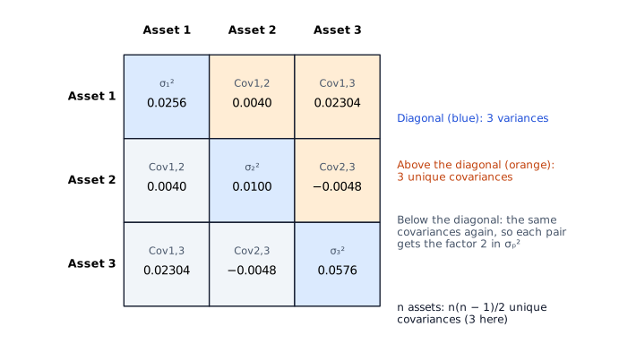
A 3 by 3 grid for Assets 1 to 3. Diagonal cells (blue) hold the variances: 0.0256, 0.0100 and 0.0576. Cells above the diagonal (orange) hold the three unique covariances: Cov1,2 = 0.0040, Cov1,3 = 0.02304 and Cov2,3 = −0.0048. Cells below the diagonal repeat the same covariances, which is why each pair gets the factor 2 in the portfolio variance. A note: with n assets there are n(n − 1)/2 unique covariances, 3 here. — The three-asset covariance matrix: variances on the diagonal, each covariance appearing twice

Each pair appears twice in the matrix, which is where the factor 2 in the cross terms comes from:

σ_{P}^{2} = (0.004096 + 0.001225 + 0.0036) + (0.00112 + 0.004608 - 0.00084) = 0.013809, σ_{P} = 11.75%

The first bracket holds the weighted variances $w_{i}^{2} σ_{i}^{2}$ and the second the terms $2 w_{i} w_{j} Cov_{i, j}$ . The result is well below the 15.9% weighted average of the three standard deviations because every correlation is below +1.

Expected portfolio variance from scenarios

A forward-looking variance can be built from economic scenarios $m$ with probabilities $p_{m}$ that sum to 1:

Portfolio return in each scenario: $R_{P, m} = \sum_{i} w_{i} R_{i, m}$ .
Expected portfolio return: $E (R_{P}) = \sum_{m} p_{m} R_{P, m}$ , which equals the weighted average of the assets' expected returns, $\sum_{i} w_{i} E (R_{i})$ .
Expected variance: $σ_{P}^{2} = \sum_{m} p_{m} [R_{P, m} - E (R_{P})]^{2}$ , then take the square root.

Example. Two equally likely scenarios give portfolio returns of 12% and 2%. Then $E (R_{P}) = 7%$ and $σ_{P}^{2} = 0.5 (5)^{2} + 0.5 (- 5)^{2} = 25$ (in %²), so $σ_{P} = 5%$ .

Large portfolios: variance approaches average covariance

For an equally weighted portfolio of $N$ assets, the exact variance is

Key concept

σ_{P}^{2} = \frac{σ ˉ ^{2}}{N} + \frac{N - 1}{N} Cov

where $σ ˉ^{2}$ is the average variance and $Cov$ the average pairwise covariance. As $N$ grows, each asset's own variance matters less and less and the portfolio variance approaches the average covariance. For a large portfolio, the approximation writes this as the average correlation times the average variance:

σ_{P}^{2} \approx ρ ˉ σ ˉ^{2}

Exam convention: for an equally weighted portfolio, a more exact variance is $σ_{P}^{2} = σ ˉ^{2} / N + (1 - 1/ N) ρ ˉ σ ˉ^{2}$ , and $ρ ˉ σ ˉ^{2}$ is its large- $N$ approximation.
Current practice: that more exact form is exact only when all assets have the same variance, because only then does $ρ ˉ σ ˉ^{2}$ equal the average covariance. In general the exact variance is $σ ˉ^{2} / N + (N - 1) / N$ times the average covariance, as above.

With unequal variances the gap can be large. For example, two assets with standard deviations of 10% and 30% and a correlation of 0.5 have a covariance of 0.015, but $ρ ˉ σ ˉ^{2} = 0.5 \times 0.05 = 0.025$ . Example. With 40 assets, an average variance of 0.05 and an average correlation of 0.25, $σ_{P}^{2} \approx 0.25 \times 0.05 = 0.0125$ , $σ_{P} \approx 11.2%$ . If all 40 assets had the same variance of 0.05, the finite- $N$ term would add $0.75 \times 0.05/40 = 0.0009$ , giving 0.0134 (11.6%).

Systematic vs. unsystematic risk

Key concept

	Unsystematic risk	Systematic risk
Other names	Unique, diversifiable, firm-specific	Market, nondiversifiable
Removed by diversification?	Yes	No
Rewarded with higher expected return?	No	Yes

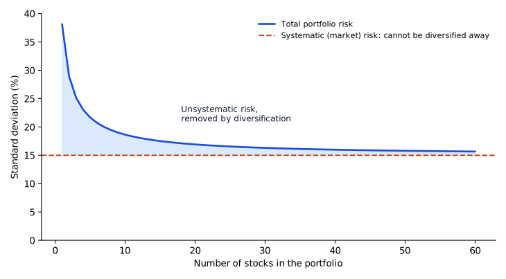
A portfolio of roughly 20 to 30 well-chosen assets captures most of the diversification benefit; beyond about 30 assets the extra benefit of each new holding is close to zero, and what remains is systematic risk.

Common exam traps

The approximation gives a variance; take the square root for standard deviation. In the 40-asset example, reading 0.0125 as 1.25% instead of taking the square root, about 11.2%.
Number of covariances is $(N^{2} - N) /2$ , not $N^{2}$ . For 20 assets, $N^{2}$ gives 400 instead of 190.
Adding assets reduces risk only to the extent that their correlations are below +1; with correlations of +1, more assets bring no diversification benefit.

Exam shortcuts

The expected portfolio return from scenarios equals $\sum w_{i} E (R_{i})$ , the assets' expected returns weighted by portfolio weight, so it can be found without the scenario portfolio returns; the variance still needs them.

Bottom line

The diversification benefit grows as correlation falls: two-asset combinations lie on a straight line at $ρ = + 1$ , bow to the left when correlation is below +1, and include one zero-risk mix at $ρ = - 1$ .
With $N$ assets the variance-covariance matrix holds $N$ variances and $(N^{2} - N) /2$ unique covariances.
Expected portfolio variance from scenarios is $\sum_{m} p_{m} [R_{P, m} - E (R_{P})]^{2}$ , with scenario probabilities that sum to 1.
An equally weighted portfolio of $N$ assets has variance $σ ˉ^{2} / N + [(N - 1) / N] Cov$ , which approaches the average covariance as $N$ grows and is approximated for a large portfolio by $ρ ˉ σ ˉ^{2}$ .
Unsystematic risk is removed by diversification and is not rewarded with higher expected return; systematic risk is not removed and is rewarded.
Roughly 20 to 30 well-chosen assets capture most of the diversification benefit, and beyond about 30 assets each new holding adds close to none.

Quick check

Question 2Core

Brookline Endowment holds an equally weighted portfolio of 50 stocks. The average variance of returns of the individual stocks is 0.09, and the average correlation between pairs of stocks is 0.30. Using the approximation for a portfolio with a large number of assets, the standard deviation of the portfolio's returns is closest to:

Show answer and explanation

Correct answer: C

For an equally weighted portfolio of many assets, the individual variances matter little and portfolio variance is approximately the average correlation times the average variance. The standard deviation is the square root of that variance.

σ_{P}^{2} \approx ρ ˉ σ ˉ^{2} = 0.30 \times 0.09 = 0.027

σ_{P} \approx 0.027 = 0.164 = 16.4%

The approximation ignores the finite- $N$ term. If every stock had the same variance of 0.09, the exact equal-weight formula would add $(1 - ρ ˉ) σ^{2} / N = 0.70 (0.09) /50 = 0.00126$ , giving $σ_{P}^{2} = 0.02826$ and $σ_{P} = 16.8%$ , still closest to 16.4%. With unequal variances, the exact result depends on the average covariance, which the given averages do not pin down, so the question asks for the approximation. The average single stock has a standard deviation of $0.09 = 30%$ ; diversification cuts this to about 16%, and the remainder is systematic risk.

Why the other options are wrong

A. 2.7% is the approximate portfolio variance (0.027) quoted as if it were the standard deviation.
B. 9.0% multiplies the average correlation by the average standard deviation ( $0.30 \times 30%$ ). The approximation multiplies the correlation by the average variance, and the square root is taken afterward.

Key takeaway For a large portfolio, $σ_{P}^{2} \approx ρ ˉ σ ˉ^{2}$ . Diversification removes unsystematic risk, but the average covariance (systematic risk) remains.

Module 8.4

The Minimum-Variance Portfolio and the Efficient Frontier

LOS 8.b — The minimum-variance portfolio and the efficient frontier

Feasible set, minimum-variance frontier and efficient frontier

Every mix of the available risky assets is a risky portfolio; together they form the set of feasible (attainable) portfolios.

The minimum-variance frontier is the set of portfolios with the lowest risk for each level of expected return. It is the left boundary of the feasible set.
The global minimum-variance portfolio is the point on that frontier with the lowest risk of all.
The efficient frontier is the set of portfolios that offer the most expected return at any given level of risk. On a graph it is the upper part of the minimum-variance frontier, beginning at the global minimum-variance portfolio and rising from there. The lower part is inefficient: another portfolio offers more return for the same risk.
Points to the left of the minimum-variance frontier, including every point above the efficient frontier, are unattainable with the available assets. Attainable points below the efficient frontier are inefficient.

Expected return (vertical, 0% to 14%) against standard deviation (horizontal, 0% to 32%). Grey dots are feasible risky portfolios lying to the right of a curved minimum-variance frontier. The global minimum-variance portfolio is at a standard deviation of 10.0% and an expected return of 6.0%. The solid upper part of the curve from that point upward is the efficient frontier; the dashed lower part is inefficient. The area above and to the left of the frontier is labeled unattainable. A straight line starts at the risk-free asset (0%, 3%) and touches the efficient frontier at the tangency (optimal risky) portfolio at about 14.2% standard deviation and 9.0% expected return; the slope of the line (Sharpe ratio) is 0.42. — Feasible portfolios, minimum-variance frontier, efficient frontier and the tangency portfolio

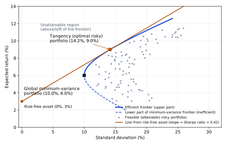
In a theoretical universe of all investable assets, the upper segment is called the Markowitz efficient frontier.

Minimum-variance portfolio of two risky assets

Key concept

w_{A} = \frac{σ _{B}^{2} - Cov _{A, B}}{σ _{A}^{2} + σ _{B}^{2} - 2 Cov _{A, B}}, w_{B} = 1 - w_{A}

When both weights are positive and the other inputs are held constant, a higher variance of an asset lowers its weight in the minimum-variance portfolio, and a lower variance raises it.

Example. With $σ_{A} = 15%$ , $σ_{B} = 25%$ and $ρ = 0.20$ , $Cov = 0.20 (0.15) (0.25) = 0.0075$ .

w_{A} = \frac{0.0625 - 0.0075}{0.0225 + 0.0625 - 0.0150} = \frac{0.0550}{0.0700} = 78.6%, w_{B} = 21.4%

The less risky asset gets the larger weight. Expected returns do not enter the formula.

Adding a risk-free asset

A risk-free asset has a return with zero variance. Exam convention: the risk-free asset has zero correlation with any risky asset. Current practice: because its return never varies, its covariance with every asset is zero and the correlation coefficient is, strictly, undefined. Either way the covariance term drops out of the portfolio variance. The straight line from the risk-free rate that just touches (is tangent to) the efficient frontier identifies the optimal risky portfolio, also called the tangency portfolio: the efficient portfolio with the highest Sharpe ratio,

Key concept

Sharpe ratio = \frac{E ( R _{P} ) - R _{f}}{σ _{P}}

Combining the risk-free asset with a risky portfolio $P$ :

E (R_{C}) = w_{P} E (R_{P}) + (1 - w_{P}) R_{f}, σ_{C} = w_{P} σ_{P}

To reach a target return, solve for the risky weight:

w_{P} = \frac{r _{target} - R _{f}}{E ( R _{P} ) - R _{f}}

Example. With $R_{f} = 4%$ , a risky portfolio with a 12% expected return and a 20% standard deviation, and a 10% target, $w_{P} = 6/8 = 0.75$ and $σ_{C} = 0.75 \times 20% = 15%$ . Weights between 0 and 100% mean lending at the risk-free rate; a risky weight above 100% means borrowing at the risk-free rate.

Portfolio optimization

Key concept

Approach	What it does
Return-constrained optimization	Minimizes risk for a given level of return
Risk-constrained optimization	Maximizes expected return for a given level of risk (finds points on the efficient frontier)
Risk-adjusted return optimization	Maximizes the Sharpe ratio

The key inputs are expected returns, volatilities (standard deviations) and asset correlations. Investor-specific factors (risk tolerance, time horizon, cash needs) and constraints such as no short selling or position limits can move weights away from the unconstrained optimum.

Common exam traps

In the minimum-variance formula, use variances ( $σ^{2}$ ) rather than standard deviations, and keep the covariance term. In the example, standard deviations give $(0.25 - 0.0075) / (0.15 + 0.25 - 0.015) = 63.0%$ instead of 78.6%.
With a risk-free asset, combined risk is just $w_{P} σ_{P}$ ; do not add a covariance term.
The risky weight for a target return is $(r_{target} - R_{f}) / (E (R_{P}) - R_{f})$ ; dividing the target by $E (R_{P})$ ignores the return on the risk-free asset. In the example, $10/12 = 0.833$ instead of 0.75.

Exam shortcuts

Expected returns do not enter the two-asset minimum-variance weights, so any expected returns given in such a question can be set aside.

Bottom line

The minimum-variance frontier holds the lowest-risk portfolio for each level of expected return, and the global minimum-variance portfolio is its point of lowest risk.
The efficient frontier is the upper part of the minimum-variance frontier from the global minimum-variance portfolio upward; points to the left of the frontier are unattainable and attainable points below the efficient frontier are inefficient.
For two risky assets, $w_{A} = (σ_{B}^{2} - Cov_{A, B}) / (σ_{A}^{2} + σ_{B}^{2} - 2 Cov_{A, B})$ and $w_{B} = 1 - w_{A}$ give the minimum-variance portfolio.
The optimal risky (tangency) portfolio is where a line from the risk-free rate touches the efficient frontier, the efficient portfolio with the highest Sharpe ratio $(E (R_{P}) - R_{f}) / σ_{P}$ .
Combining the risk-free asset with portfolio $P$ gives $E (R_{C}) = w_{P} E (R_{P}) + (1 - w_{P}) R_{f}$ and $σ_{C} = w_{P} σ_{P}$ , with $w_{P} = (r_{target} - R_{f}) / (E (R_{P}) - R_{f})$ for a target return and a weight above 100% meaning borrowing at the risk-free rate.
Return-constrained optimization minimizes risk for a given return, risk-constrained optimization maximizes expected return for a given risk, and risk-adjusted return optimization seeks the highest Sharpe ratio.

Module 8.5

Risk Aversion

LOS 8.c — Risk aversion, utility and indifference curves

Assumptions behind optimal portfolio choice

Investors are rational and risk averse; they maximize satisfaction (utility) and prefer more return and less risk.
A single-period time horizon.
No taxes or transaction costs.
Investors can borrow and lend at a constant risk-free rate.

Three attitudes toward risk

Key concept

Attitude	Behavior	Coefficient $A$	Indifference curves
Risk seeking	Prefers an uncertain outcome to a certain one with the same expected value; may accept a lower expected return (e.g., casino gambling)	$A < 0$	Slope downward
Risk neutral	Indifferent between a gamble and a sure amount with the same expected value; cares only about return	$A = 0$	Flat (horizontal)
Risk averse	Prefers the certain outcome; needs extra return to bear extra risk	$A > 0$	Slope upward

A fair gamble (expected gain of zero) raises the expected utility of a risk-seeking investor, leaves a risk-neutral investor indifferent, and lowers the utility of a risk-averse investor. Most real-world investors are risk averse; risk neutrality is a useful theoretical case (e.g., large institutions making many small trades whose variance averages out).

Utility function

A common utility function is

Key concept

U = E (r) - \frac{1}{2} A σ^{2}

where $A$ is the investor's coefficient of risk aversion and $σ^{2}$ the variance of returns (use decimals). A higher $A$ means a bigger utility penalty for risk. Portfolio theory assumes every investor is risk averse ( $A > 0$ ). Research suggests $A$ typically lies between 2 and 3 and is rarely below 1. Mean-variance utility, $U_{P} = U [E (R_{P}), σ_{P}]$ , depends only on expected return and risk and ignores other factors such as total wealth.

Example. With $A = 4$ , an expected return of 10% and a standard deviation of 15%, $U = 0.10 - 0.5 (4) (0.0225) = 0.055$ , i.e., 5.5%. The investor would be equally happy with a certain 5.5% return.

Risk tolerance is the willingness to accept risk for higher expected return; it is the inverse of risk aversion and can change with age, wealth and economic conditions, and differs across countries and cultures. Absolute risk aversion looks at how utility changes with extra risk holding wealth constant; relative risk aversion looks at how the share of wealth put at risk changes as wealth changes.

Indifference curves

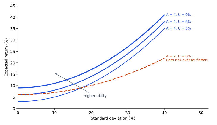
An indifference curve plots the risk–return combinations that give an investor the same expected utility. For a risk-averse investor the curves slope upward and are convex; curves higher and to the left represent higher utility. The slope measures how much extra return is required per unit of extra risk:

A more risk-averse (less risk-tolerant) investor has steeper curves.
A less risk-averse (more risk-tolerant) investor has flatter curves.

Indifference curves: higher curves give higher utility, and a less risk-averse investor has flatter curves (illustrative utility levels)

Common exam traps

The utility function uses the variance rather than the standard deviation, together with the factor $\frac{1}{2}$ . In the example, using the standard deviation gives $0.10 - 0.5 (4) (0.15) = - 0.20$ and dropping the $\frac{1}{2}$ gives 0.010, instead of 0.055.
The highest expected return or the lowest risk is not necessarily the highest-utility choice; compute $U$ for each.

Bottom line

Optimal portfolio theory assumes rational, risk-averse investors who maximize utility, a single-period horizon, no taxes or transaction costs, and borrowing and lending at a constant risk-free rate.
A risk-seeking investor has $A < 0$ and downward-sloping indifference curves, a risk-neutral investor has $A = 0$ and flat curves, and a risk-averse investor has $A > 0$ and upward-sloping curves.
Utility is $U = E (r) - \frac{1}{2} A σ^{2}$ with the variance in decimals, so a higher coefficient of risk aversion $A$ means a bigger penalty for risk.
Risk tolerance, the inverse of risk aversion, can change with age, wealth and economic conditions.
A risk-averse investor's indifference curves slope upward and are convex, curves higher and to the left give higher utility, and a more risk-averse investor has steeper curves.

Quick check

Question 3Core

An adviser measures a client's utility with the function $U = E (r) - \frac{1}{2} A σ^{2}$ and estimates the client's coefficient of risk aversion, $A$ , at 3. Based on the table below, which fund gives this client the highest utility?

Funds under consideration

Fund	Expected return	Standard deviation of returns
Northgate Growth Fund	11%	20%
Westbury Balanced Fund	8%	12%
Eastholm Income Fund	6%	5%

Show answer and explanation

Correct answer: B

Utility rewards expected return and penalizes variance in proportion to the coefficient of risk aversion. Computing the utility of each fund (with returns and standard deviations in decimals and the standard deviation squared) shows that the balanced fund offers the best trade-off for this client.

U = E (r) - \frac{1}{2} (3) σ^{2} = E (r) - 1.5 σ^{2}

Fund	$E (r)$	$σ^{2}$	$U$
Northgate Growth	0.11	0.0400	$0.11 - 0.0600 = 0.0500$
Westbury Balanced	0.08	0.0144	$0.08 - 0.0216 = 0.0584$
Eastholm Income	0.06	0.0025	$0.06 - 0.00375 = 0.05625$

Westbury Balanced has the highest utility (5.84%).

Why the other options are wrong

A. Northgate Growth has the highest expected return, but its large variance creates the biggest utility penalty ( $1.5 \times 0.04 = 0.06$ ), leaving a utility of only 5.00%.
C. Eastholm Income has the lowest risk and is the choice that results if the standard deviation is used instead of the variance in the penalty term. With the variance, its utility (5.625%) is slightly below that of the balanced fund.

Key takeaway Use $σ^{2}$ (in decimals) and the $\frac{1}{2}$ in the utility function; neither the highest return nor the lowest risk is automatically the best choice.

Module 8.6

Capital Allocation Line and Capital Market Line

LOS 8.c — Capital allocation line, optimal portfolio and the capital market line

The capital allocation line (CAL)

Combining a risky portfolio with the risk-free asset (assuming zero risk for the risk-free asset, a risky portfolio whose return and risk exceed the risk-free rate, only these two assets available, and unlimited borrowing and lending at the risk-free rate) gives a straight line in risk–return space:

Key concept

E (R_{C}) = R_{f} + [\frac{E ( R _{P} ) - R _{f}}{σ _{P}}] σ_{C}

This is the risky portfolio's capital allocation line (CAL). It starts at the risk-free rate on the vertical axis, and its slope is the risky portfolio's Sharpe ratio. Points between the intercept and the risky portfolio involve lending (a positive weight in the risk-free asset); points beyond it involve borrowing.

Example. Let $R_{f} = 3%$ ; the tangency portfolio has an expected return of 10.2% and a standard deviation of 18% (Sharpe ratio $= 7.2/18 = 0.40$ ). A client with 40% in the risky portfolio has $E (R) = 0.40 (10.2%) + 0.60 (3%) = 5.88%$ and $σ = 0.40 (18%) = 7.2%$ ; check with the CAL: $3% + 0.40 (7.2%) = 5.88%$ . A client who borrows 30% of wealth at 3% and puts 130% in the risky portfolio has $E (R) = 1.30 (10.2%) - 0.30 (3%) = 12.36%$ and $σ = 1.30 (18%) = 23.4%$ ; check: $3% + 0.40 (23.4%) = 12.36%$ . Both portfolios lie on the same line.

Choosing the optimal portfolio

The investor's optimal portfolio is the point where the CAL touches the highest attainable indifference curve. Higher curves would be better but cannot be reached; lower curves are dominated.

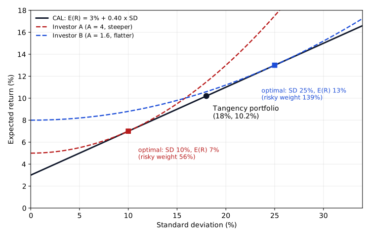
Optimal portfolios on a CAL for a more and a less risk-averse investor

In the figure, the more risk-averse Investor A (steeper indifference curves) reaches the highest attainable curve at a standard deviation of 10% (about 56% in the risky portfolio, the rest lent at the risk-free rate). The less risk-averse Investor B (flatter curves) chooses 25% (about 139% in the risky portfolio, financed partly by borrowing). Both points lie on the same CAL: risk aversion changes where on the line an investor sits, while the slope of the line stays the same.

The capital market line (CML)

The capital market line (CML) is the special CAL whose risky portfolio is the market portfolio, which holds all risky assets weighted by market value:

E (R_{P}) = R_{f} + [\frac{E ( R _{M} ) - R _{f}}{σ _{M}}] σ_{P}

The market portfolio sits on the efficient frontier and is mean-variance efficient (the highest Sharpe ratio possible). The mutual fund theorem states that every investor can obtain an efficient portfolio by combining the risk-free asset with the market portfolio; investors differ only in how much of each they hold.

Key concept

	CAL	CML
Risky portfolio	Any risky portfolio (e.g., the investor's own tangency portfolio)	The market portfolio
Expectations	Heterogeneous — each investor can have a different CAL	Homogeneous — one CML for all investors
Slope	Sharpe ratio of that risky portfolio	Sharpe ratio of the market portfolio

In practice a portfolio of "all risky assets" cannot be held, so a broad market index is used as the proxy.

Common exam traps

Every portfolio on a CAL has the same Sharpe ratio as that CAL's risky portfolio, however much is lent or borrowed.
The mutual fund theorem combines the risk-free asset with the market portfolio specifically; another efficient portfolio or the minimum-variance portfolio does not qualify.
Owning "about 30 stocks" diversifies away most unsystematic risk; that rule of thumb is a different idea from the mutual fund theorem.

Exam shortcuts

Every portfolio on a CAL with a positive allocation to the risky portfolio has the Sharpe ratio of that risky portfolio, however much is lent or borrowed, so its Sharpe ratio can be read from the risky portfolio directly.

Bottom line

Under its assumptions (a riskless risk-free asset, a risky portfolio with return and risk above the risk-free rate, only these two assets, and unlimited borrowing and lending at the risk-free rate), the CAL is $E (R_{C}) = R_{f} + [(E (R_{P}) - R_{f}) / σ_{P}] σ_{C}$ , with intercept $R_{f}$ and slope equal to the risky portfolio's Sharpe ratio.
Points on the CAL between the intercept and the risky portfolio involve lending at the risk-free rate, and points beyond the risky portfolio involve borrowing.
An investor's optimal portfolio is where the CAL touches the highest attainable indifference curve; a more risk-averse investor chooses a lower-risk point on the same line.
The CML is the CAL whose risky portfolio is the market portfolio, which holds all risky assets weighted by market value and is mean-variance efficient.
Under the mutual fund theorem, every investor can obtain an efficient portfolio by combining the risk-free asset with the market portfolio.
A CAL allows heterogeneous expectations, so each investor can have a different CAL, while the CML assumes homogeneous expectations and is the same for all investors.

Module 8.7

The Capital Asset Pricing Model

LOS 8.c — Systematic risk, beta and the capital asset pricing model (CAPM)

Only systematic risk is priced

The market portfolio holds every risky asset, so all unsystematic risk has been diversified away within it and only systematic risk remains (Module 8.3). Since unsystematic risk can be removed at no cost, the market rewards investors only for bearing systematic risk, and the CAPM prices assets on that basis.

Portfolio standard deviation (%) against the number of equally weighted stocks, from 1 to 60. The total-risk curve starts near 38% for one stock, falls steeply to about 19% at 10 stocks and then flattens toward a dashed horizontal line at 15%, the systematic (market) risk that cannot be diversified away. The shaded gap between the curve and the line is unsystematic risk, removed by diversification. — Diversification: portfolio risk falls toward systematic risk as stocks are added (illustrative figures)

Return-generating models and the CAPM

Return-generating models estimate expected returns from one or more factors (macroeconomic factors such as GDP growth or inflation, or fundamental factors such as earnings growth or firm size). The capital asset pricing model (CAPM) is a single-factor model: expected return depends only on exposure to systematic risk.

The CAPM assumes homogeneous expectations; investors hold efficient portfolios that maximize their expected utility; investors are price takers; and markets are in equilibrium (no mispriced assets).

Key concept

E (R_{i}) = R_{f} + β_{i} [E (R_{M}) - R_{f}]

$E (R_{M}) - R_{f}$ is the market risk premium, the extra return expected for holding the market instead of the risk-free asset.

Beta

Beta measures an asset's sensitivity to market (systematic) risk:

Key concept

β_{i} = \frac{Cov ( R _{i} , R _{M} )}{σ _{M}^{2}} = \frac{ρ _{i, M} σ _{i} σ _{M}}{σ _{M}^{2}} = \frac{ρ _{i, M} σ _{i}}{σ _{M}}

The market portfolio has a beta of 1.

Exam convention: a beta above 1 indicates an expected return above the market's, and a beta below 1 an expected return below it.
Current practice: this holds only when the market risk premium is positive; with a negative premium the ordering reverses.

Beta can be estimated by regression (see the reading on simple linear regression).

Example. With $ρ_{i, M} = 0.5$ , $σ_{i} = 36%$ and $σ_{M} = 20%$ , $β = 0.5 \times 36/20 = 0.90$ . A stock can be almost twice as volatile as the market, as here, and still have a beta below 1 if its correlation with the market is low.

The security market line (SML)

The security market line (SML) is the graph of the CAPM: expected return on the vertical axis, beta on the horizontal axis, intercept $R_{f}$ , slope equal to the market risk premium.

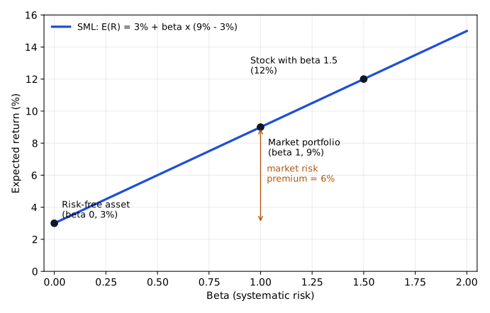
Expected return (vertical) against beta (horizontal, 0 to 2). The SML starts at the risk-free rate of 3% at beta 0, passes through the market portfolio at beta 1 and 9%, and through a stock with beta 1.5 at 12%. The vertical distance between 3% and 9% at beta 1 is labeled market risk premium = 6%. — The security market line

Example (from the figure). With $R_{f} = 3%$ , $E (R_{M}) = 9%$ and $β = 1.5$ , $E (R) = 3% + 1.5 (6%) = 12%$ .

Key concept

	CML	SML
Horizontal axis	Total risk (standard deviation)	Systematic risk (beta)
Applies to	Efficient portfolios only	Any asset or portfolio
Slope	Market Sharpe ratio	Market risk premium

Limitations of portfolio theory

Asset returns are not normally distributed (skewness, kurtosis); correlations are unstable, especially in market stress; markets are less than perfectly efficient; models are very sensitive to estimation error; the future may not look like the past. Practical constraints ignored by the theory include transaction costs from rebalancing and taxes. Taxes on distributions and on capital appreciation differ across portfolios and can change the optimal portfolio, and realizing capital losses to offset capital gains changes after-tax, risk-adjusted realized returns.

Common exam traps

If the question gives the market risk premium, multiply it by beta directly; if it gives the market return, subtract $R_{f}$ first. In the SML example, using the 9% market return as the premium gives $3% + 1.5 (9%) = 16.5%$ instead of 12%.
Do not forget to add the risk-free rate back. In the SML example, $1.5 \times 6% = 9%$ instead of 12%.
Beta uses the correlation and both standard deviations: $β = ρ σ_{i} / σ_{M}$ rather than $σ_{i} / σ_{M}$ . In the example, $36/20 = 1.80$ instead of 0.90.

Bottom line

Because unsystematic risk can be diversified away at no cost, the market rewards investors only for bearing systematic risk.
The CAPM is a single-factor model, $E (R_{i}) = R_{f} + β_{i} [E (R_{M}) - R_{f}]$ , that assumes homogeneous expectations, utility-maximizing investors holding efficient portfolios, price takers and markets in equilibrium.
Beta is $Cov (R_{i}, R_{M}) / σ_{M}^{2} = ρ_{i, M} σ_{i} / σ_{M}$ , and the beta of the market portfolio is 1.
Exam convention: a beta above 1 indicates an expected return above the market's and a beta below 1 one below it; current practice: this ordering holds only when the market risk premium is positive.
The SML plots expected return against beta with intercept $R_{f}$ and slope equal to the market risk premium and applies to any asset, while the CML plots against total risk and applies only to efficient portfolios.
Portfolio theory is limited by non-normal returns, unstable correlations, imperfectly efficient markets, sensitivity to estimation error and a future that may differ from the past, and it ignores transaction costs and taxes.

Quick check

Question 4Core

Using the capital asset pricing model (CAPM) and the data in the table below, the expected return on Gorham Textiles shares is closest to:

Inputs for Gorham Textiles

Input	Value
Beta of Gorham Textiles	0.8
Market risk premium	6%
Risk-free rate	3%

Show answer and explanation

Correct answer: A

Under the CAPM, an asset's expected return equals the risk-free rate plus beta times the market risk premium. The market risk premium is given directly, so it is multiplied by beta without subtracting the risk-free rate again.

E (R_{i}) = R_{f} + β_{i} [E (R_{M}) - R_{f}] = 3% + 0.8 (6%) = 3% + 4.8% = 7.8%

Why the other options are wrong

B. 5.4% treats 6% as the market return and subtracts the risk-free rate again: $3% + 0.8 (6% - 3%)$ . The 6% is already the market risk premium.
C. 4.8% is only the asset's risk premium, $0.8 \times 6%$ ; the risk-free rate must be added.

Key takeaway Check whether the question gives the market return or the market risk premium before plugging into the CAPM.

This reading has 23 questions in the full bank. Practice all of them.

Key Takeaways

No rebalancing means the weights drift: recompute each weight from start-of-period market values before weighting the period's returns.
For a large portfolio, $σ_{P}^{2} \approx ρ ˉ σ ˉ^{2}$ . Diversification removes unsystematic risk, but the average covariance (systematic risk) remains.
Use $σ^{2}$ (in decimals) and the $\frac{1}{2}$ in the utility function; neither the highest return nor the lowest risk is automatically the best choice.
Check whether the question gives the market return or the market risk premium before plugging into the CAPM.