Quantitative Methods · Reading 7
Null Hypothesis
CFA Level I · Quantitative Methods · Reading 7: Estimation and Hypothesis Testing · about 1 h 8 min
What you'll learn
- LOS 7.a Explain the central limit theorem and use it to build confidence intervals, measure parametric VaR and choose among sampling methods.
- LOS 7.b Construct and interpret parametric tests of differences between means, mean differences, a single variance, two variances and a correlation coefficient; recognize p-values and p-hacking.
- LOS 7.c Compare parametric and nonparametric tests, identify when a nonparametric test is appropriate, and construct and interpret the Spearman rank correlation test and the chi-square test of independence.
Module 7.1
The Central Limit Theorem, Confidence Intervals, and Sampling
This reading moves from a sample to the population: how sample means behave under the central limit theorem, how confidence intervals are built and how samples are drawn. It then sets out the steps of a hypothesis test, the test statistic for each parametric test, the two types of error, and the nonparametric tests used for ranks and categories.
LOS 7.a — The central limit theorem, confidence intervals and sampling
The central limit theorem (CLT)
A population parameter such as or is a fixed number, usually unknown. A sample statistic such as or is computed from the sample actually drawn, so it would take a different value in another sample: it is itself a random variable. The distribution of its values over all possible samples of the same size is the statistic's sampling distribution.
Take many simple random samples of size from a population with mean and a finite variance . The central limit theorem says that the sampling distribution of the sample mean becomes approximately normal as grows, whatever the shape of the population itself (skewed, flat, lumpy):
Key concept
Three consequences follow:
- The mean of all possible sample means equals the population mean: .
- The variance of the sample mean is the population variance divided by the sample size, , which shrinks as rises.
- The CLT describes the distribution of the sample mean. Individual observations keep the population's shape, and the CLT says nothing about the distribution of the sample standard deviation.
Standard error and sampling error
Sampling error is the difference between a sample statistic and the population parameter it estimates (e.g., ). Its typical size is the standard error of the sample mean:
Key concept
When is unknown, replaces it, and the result is an estimate of the standard error. The standard deviation describes how widely individual observations scatter around the mean, and a larger sample does not make it smaller. The standard error describes how precisely estimates .
Calculator. From raw data, enter the observations in the DATA worksheet, read the sample standard deviation in the STAT worksheet (1-V), and divide it by .
Example. A population of quarterly returns has . With , ; quadrupling the sample to 144 halves the standard error to 1.5%.
Desirable properties of an estimator
| Property | Meaning |
|---|---|
| Unbiased | Expected value of the estimator equals the parameter (the sample mean is unbiased for ). |
| Efficient | Smallest sampling variance among unbiased estimators. An estimator that is both unbiased and efficient is the minimum variance unbiased estimator (MVUE); the unbiased estimator with the lowest variance among those formed as a linear combination of the sample data is the best linear unbiased estimator (BLUE). |
| Consistent | Accuracy improves as increases (standard error falls toward zero). |
| Robust | Not sensitive to outliers or non-normal data (the sample mean is not robust). |
Confidence intervals
A point estimate is a single value (e.g., ). A confidence interval is a range built around it that contains the true parameter with a stated confidence level , where is the significance level:
| Situation | Reliability factor | Interval for |
|---|---|---|
| Normal population, known | ||
| Normal (or approximately normal) population, unknown (use ); required when is small | with df | |
| unknown, large sample (), any population shape (CLT) | preferred; acceptable as an approximation | , or as a large-sample approximation |
Two-tailed z reliability factors are 1.65 for 90% (1.645 before rounding), 1.96 for 95% and 2.58 for 99% (2.576 before rounding). Three things set the width of an interval. A higher confidence level (a larger reliability factor) widens it, a more dispersed population widens it, and a larger sample (a smaller standard error) narrows it.
The Student's t-distribution is bell-shaped and symmetric but has fatter tails than the normal; its critical values are larger than z-values (wider intervals) and fall toward the z-value as degrees of freedom rise. For a 95% interval, the t reliability factor is 2.228 with 10 df, 2.086 with 20 df and 2.042 with 30 df, against 1.96 for z. Select a t-value from a table using the area in one tail ( for a two-sided interval) and degrees of freedom.
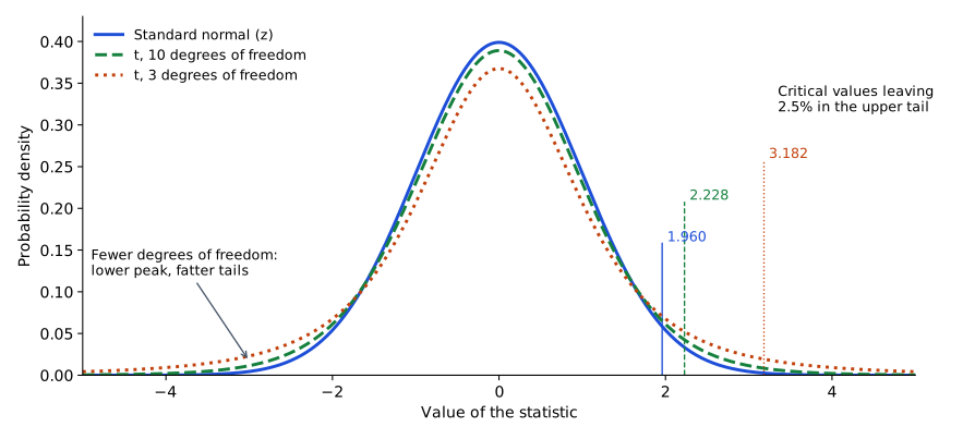
Example (σ known). With 49 observations, and , the standard error ; 95% interval to . Example (σ unknown, small sample). Ten observations from a population assumed normal give . The 95% reliability factor is rather than 1.96. If a small sample comes from a clearly non-normal population, neither a t- nor a z-interval is reliable.
Value at risk (VaR) — a one-tailed interval
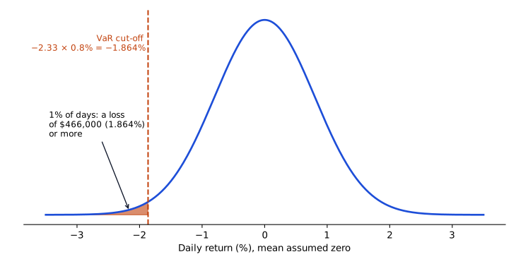
Value at risk is the loss that will be equaled or exceeded with a stated (small) probability over a given period. "The daily 1% VaR is $0.47 million" means a 1% chance on any day of losing $0.47 million or more (equivalently, 99% confidence that the loss will be smaller). VaR is the minimum loss at the stated probability; larger losses remain possible, so it is not the worst possible loss.
Under the parametric method (normal returns, mean return assumed to be zero):
with the whole in one tail: , (1.645 before rounding), . With in percent and the portfolio value in dollars, VaR is a dollar loss; dropping the portfolio value gives VaR as a percentage of the portfolio. Example. For a $25 million portfolio with daily , the daily 1% VaR , or 1.864% of the portfolio.
Drawbacks: returns are often skewed/fat-tailed, parameters change over time, history may not reflect new conditions, and it handles nonlinear payoffs (options) poorly.
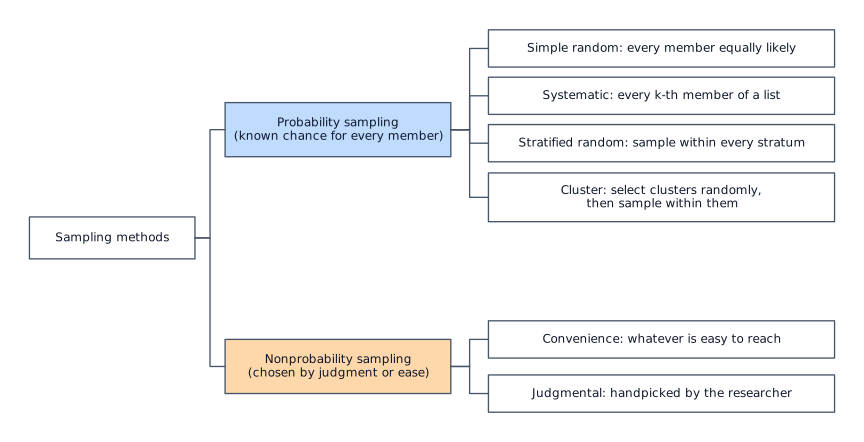
Sampling methods
| Family | Method | How the sample is drawn |
|---|---|---|
| Probability sampling (every member has a known, nonzero chance) | Simple random sampling | Every member has the same chance of selection, through random draws from the full list (so every possible sample of size is equally likely). Equal individual chances alone are not enough; a systematic sample with a random start also gives every member the same chance. |
| Systematic sampling | Select every -th member of the population list. | |
| Stratified random sampling | Split the population into strata by a characteristic (sector, size, rating); draw a random sample within each stratum, usually in proportion to its weight in the population; pool the results. | |
| Cluster sampling | Split into clusters that each resemble the population; randomly select clusters and sample within them. The CLT applies if the clusters are large enough. | |
| Nonprobability sampling | Convenience sampling | Use whatever is easy to reach (e.g., colleagues at one office); cheap but likely unrepresentative. |
| Judgmental sampling | The researcher handpicks elements using experience and judgment; may import the researcher's bias, but expert judgment can help on complex research questions. |
Probability sampling is generally more accurate; nonprobability sampling is cheaper. Stratified and cluster sampling both split the population into groups. Stratified sampling draws from every group, so the sample keeps the population's mix across groups; cluster sampling uses only some groups, so differences between groups can be lost.
The CLT does not rescue a non-representative sample.
Common exam traps
- The CLT requires a finite variance and a large , where is the size of each sample; drawing more samples of the same small size does not help. It does not require a normal population, and it describes the sample mean.
- The standard error divides by rather than by . With and , dividing by 36 gives 0.5% instead of 3%.
- Two-sided 95% uses 1.96; one-tailed 5% (VaR) uses 1.645. Always check how many tails. In the VaR example, the two-tailed 1% value 2.58 would give $516,000 instead of $466,000.
- "Random draws, then keep every second one drawn" is still simple random sampling, because keeping fixed positions of an already random sequence leaves the selection purely random. Systematic sampling means every -th item of a fixed, ordered population list.
- Grouping first and sampling within each group is stratified sampling; handpicking is judgmental sampling; choosing what is easiest to reach is convenience sampling.
Exam shortcuts
- Quadrupling the sample size halves the standard error.
- Reliability factors: two-tailed 90%, 95% and 99% use 1.65, 1.96 and 2.58; one-tailed 10%, 5% and 1% (VaR) use 1.28, 1.65 and 2.33.
- A higher confidence level widens an interval and a larger sample narrows it, which rules out answer choices that move the wrong way.
Bottom line
- By the central limit theorem, the mean of samples of size from any population with a finite variance is approximately normal with mean and variance .
- The sample mean's standard error is , or when is unknown.
- A confidence interval is the point estimate ± reliability factor × standard error, with a t reliability factor and df when is unknown.
- A desirable estimator is unbiased, efficient and consistent.
- Parametric VaR is portfolio value with the whole in one tail; it is the minimum loss at the stated probability, not the worst possible loss.
- Simple random, systematic, stratified and cluster sampling are probability methods; convenience and judgmental sampling are nonprobability methods.
Quick check
A fixed-income analyst splits the universe of investment-grade corporate bonds into five credit-rating buckets. From each bucket she randomly draws a number of bonds proportional to that bucket's share of the universe and then combines the draws into one sample of 400 bonds. Her approach is best described as:
Show answer and explanation
Correct answer: C
The analyst first divides the population into subgroups (strata) using a classification scheme (here, credit rating) and then draws a random sample within each stratum, pooling the results. That is stratified random sampling. Sampling each stratum in proportion to its weight ensures that the rating mix of the sample mirrors the population.
Why the other options are wrong
- A. In simple random sampling every bond in the universe would have the same chance of selection from a single, undivided list; here the population is first split into rating buckets and each bucket is sampled separately.
- B. Systematic sampling selects every k-th member of an ordered population list. The analyst makes random draws inside each rating bucket instead.
Key takeaway Dividing the population into groups first and then sampling randomly within every group is stratified random sampling.
Module 7.2
Hypothesis Tests of the Population Mean
LOS 7.b — Hypothesis tests of a population mean
What a hypothesis test does
A hypothesis is a claim about what value a population parameter takes (e.g., "the mean daily return of this strategy is zero"). A sample is used to decide whether the data give enough evidence to reject that statement.
- Parametric tests make assumptions about the population's distribution and test its parameters (mean, variance).
- Nonparametric tests make few distributional assumptions or test things that are not parameters (ranks, category counts); Module 7.4 covers them.
The four steps
- State the null hypothesis and the alternative hypothesis .
- Identify the test statistic and its distribution.
- Specify the significance level .
- Establish the decision rule (the critical value(s)) and compare.
Hypotheses. The null is usually the claim the researcher hopes to reject, and it always contains the equality (=, ≤ or ≥). The alternative is what the researcher wants to find evidence for. The two are mutually exclusive and exhaustive.
| Evidence sought | Test | Rejection region | ||
|---|---|---|---|---|
| Mean differs from (either direction) | two-tailed test | both tails, each | ||
| Mean is greater than | one-tailed test | right tail, all of | ||
| Mean is less than | one-tailed test | left tail, all of |
Test statistic for a mean
The test statistic measures how many standard errors the sample mean lies from the hypothesized value:
Key concept
When is used and the population is normal (or approximately normal), the statistic follows a t-distribution with degrees of freedom; with a large sample () the CLT makes the t-test approximately valid even for a non-normal population, and the z-statistic (standard normal) is an acceptable approximation. A small sample from a clearly non-normal population supports neither test. When the population is normal and its variance is known, the statistic uses and follows the standard normal distribution at any sample size; z critical values have no degrees of freedom. The sign matters: a negative statistic means the sample mean is below .
Critical z-values (exam values; three-decimal values in parentheses):
Key concept
| Significance level | Two-tailed test | One-tailed test |
|---|---|---|
| 10% | ±1.65 (1.645) | 1.28 (1.282) |
| 5% | ±1.96 | 1.65 (1.645) |
| 1% | ±2.58 (2.576) | 2.33 (2.326) |
Decision rule. Reject if the test statistic falls in the rejection region (beyond the critical value); otherwise fail to reject . The null is never "accepted"; failing to reject means only that the data were not strong enough to reject it. The confidence level is . For a two-tailed test the rule is equivalent to a confidence interval: is rejected when the sample mean falls outside the interval (critical value standard error) built around the hypothesized value.
The critical value depends on three things: the distribution of the test statistic (z, or t with its degrees of freedom), the significance level, and whether the test is one-tailed or two-tailed. At , for example, a statistic of 1.75 exceeds the critical value of a right-tailed test (1.65) but not that of a two-tailed test (1.96), so the two tests reach different decisions.
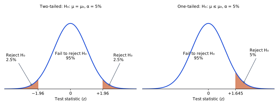
Example. A sample of 81 daily returns has and ; the test is , two-tailed, at . The standard error is and the statistic is . Because 2.10 exceeds 1.96, is rejected. At (critical value ±2.58), would not be rejected.
What moves the statistic. For a sample mean above , the statistic (and the chance of rejection) rises when the sample mean rises, the standard deviation falls or the sample size rises (smaller standard error).
Type I and Type II errors, power
| is true | is false | |
|---|---|---|
| Reject | Type I error (false positive); probability = | Correct decision; probability = power of the test |
| Fail to reject | Correct decision; probability = (confidence level) | Type II error (false negative); probability = |
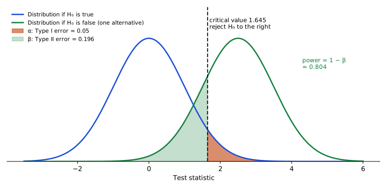
- The significance level is the probability of a Type I error, that is, of rejecting a true null by chance.
- The power of a test is the probability of correctly rejecting a false null: power .
- Only one error type can occur in a given test: a Type I error needs a true null, a Type II error needs a false null.
- Trade-off: with the sample size and the test statistic unchanged, lowering (e.g., from 5% to 1%) raises the probability of a Type II error and lowers power; raising power in that setting means accepting a higher . A lower also means a larger critical value, so the matching confidence interval is wider.
- Exam convention: for a given , power can be raised only by increasing the sample size, which lowers the probability of a Type II error while the probability of a Type I error stays at . Current practice: at a given , less noisy data (a lower standard deviation) or a more powerful test statistic also raise power.
- The chance of a Type II error depends jointly on and the sample size, but the relation is not simple and that probability is hard to compute in practice. When several test statistics could be used for the same hypothesis, the most powerful one is normally preferred.
Example. A spam filter tests : "this message is legitimate." Sending a legitimate message to the junk folder rejects a true null (Type I); letting spam through fails to reject a false null (Type II).
Worked example: a confidence interval and a one-tailed test
A sample of 64 monthly returns has a mean of 0.85% and a standard deviation of 2.4%. The population standard deviation is unknown. Build a 95% confidence interval for the mean, then test at the 5% level whether the mean return is above 0.5%.
Step 1. Standard error .
Step 2. 95% confidence interval. With , the z reliability factor is an acceptable approximation: , from 0.262% to 1.438%. The t reliability factor with 63 df is 1.998, which gives a slightly wider interval, from 0.251% to 1.449%.
Step 3. Test whether the mean return is above 0.5% at the 5% level: and . The test is one-tailed, so all of the 5% is in the right tail and the critical value is 1.65 (1.669 for t with 63 df).
Step 4. Test statistic .
Step 5. 1.17 is below the critical value, so is not rejected: the sample does not show a mean return above 0.5%.
Step 6. If the true mean is above 0.5%, this decision is a Type II error. A Type I error cannot have occurred, because was not rejected.
Common exam traps
- A 5% significance level corresponds to a 95% confidence level; "95% significance" misreads the two terms.
- The probability of a Type I error in a two-tailed 5% test is 5%; 2.5% is the area in each tail.
- Power is ; is the confidence level.
- for a two-tailed test uses "≠"; "<" or ">" signals a one-tailed test.
- Check which tail: for , the null is rejected only when the statistic is below the negative critical value.
- A two-tailed 10% test and a one-tailed 5% test share the critical value 1.65, because both place 5% in the tail beyond it.
Exam shortcuts
- The hypothesis that contains the equality sign is .
- A two-tailed 10% test and a one-tailed 5% test share the critical value 1.65.
- For a two-tailed test, is rejected when the sample mean falls outside critical value × standard error, so a confidence interval answers the test directly.
Bottom line
- always contains the equality and is usually the claim the researcher hopes to reject; is the claim the researcher seeks evidence for.
- The test statistic is (sample mean − ) ÷ standard error, following a t-distribution with df when is used.
- is rejected when the statistic falls beyond the critical value; otherwise the decision is to fail to reject, and the null is never accepted.
- A Type I error rejects a true null with probability ; a Type II error fails to reject a false null with probability ; power is .
- With the sample size unchanged, a lower makes a Type II error more likely and reduces power.
Quick check
A researcher keeps her sample size unchanged but tightens the significance level of her test from 5% to 1%. As a result, the probability of:
Show answer and explanation
Correct answer: A
Lowering the significance level lowers the probability of a Type I error. For a fixed sample size, the rejection region shrinks, so a false null is less likely to be rejected: the probability of a Type II error rises and the power of the test falls.
Why the other options are wrong
- B. Rejecting a true null is a Type I error, whose probability is the significance level; it falls from 5% to 1%.
- C. Failing to reject a false null is a Type II error; its probability increases when α is reduced with no change in sample size. A null is never 'accepted'; a test can only fail to reject it.
Key takeaway With fixed, a lower means a higher and a lower power.
Module 7.3
Other Parametric Hypothesis Tests
LOS 7.b — Other parametric hypothesis tests
Every test below uses the same four steps as the test of a single mean (hypotheses, test statistic, significance level, decision rule). What changes is the test statistic and the distribution its critical values come from.
Summary of the tests
Key concept
| What is tested | Test statistic | Distribution / degrees of freedom | Key assumptions |
|---|---|---|---|
| Single mean | t, (z if is large) | normal population, or a large sample | |
| Difference between means (independent samples) | , with pooled variance | t, | independent samples, normal populations, equal (unknown) population variances |
| Mean difference (paired comparisons test, dependent samples) | t, (n = number of pairs) | paired observations, normal differences | |
| Single variance | chi-square, | normal population | |
| Equality of two variances | (larger variance on top) | F, and | normal populations, independent samples |
| Correlation equals zero | t, | normally distributed variables |
Difference between means vs. paired comparisons
- Independent samples (e.g., returns of small-cap funds vs. returns of large-cap funds): test with the difference-in-means t-test, df . These df belong to the pooled version, which assumes the two population variances are equal and combines both samples into one variance estimate . A test that does not assume equal variances uses the unpooled standard error , with df from a separate (Welch) approximation that are usually smaller than . When , the pooled and unpooled standard errors are identical, and when the sample variances are similar the two t-values are close.
- Exam convention: the difference-in-means statistic may be shown with the unpooled standard error and still be compared with a t critical value for df.
- Current practice: df go with the pooled standard error (equal variances assumed); the unpooled (Welch) test uses fewer df.
- Dependent samples (the same members measured twice, e.g., each fund's return before and after a fee cut): compute the difference for each pair, then run a single-mean test on those differences. This is the paired comparisons test, with df .
Example (independent samples). , , ; , , . Assuming equal population variances, and ; df = 54, 5% two-tailed critical value 2.005, so the null of equal means is not rejected. (The unpooled standard error would give ; the conclusion is the same.) Example (paired). With 16 pairs, and , . This exceeds , so a zero mean difference is rejected.
Test of a single variance (chi-square)
The chi-square distribution is asymmetric (right-skewed) and bounded below by zero. For a two-tailed test at , find a lower critical value (area to its right) and an upper one (area to its right). Example. With 21 observations, and , . With 20 df and the critical values are 9.591 and 34.170, so the null is not rejected.
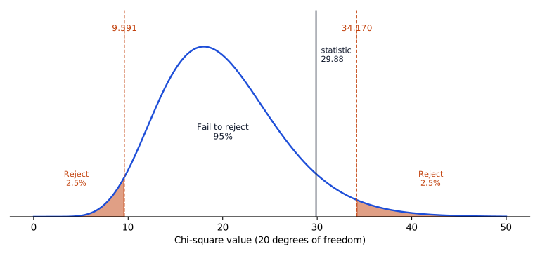
A hypothesis about a standard deviation is written in terms of the variance. With returns in decimals, a claim that is below 3% becomes versus , and only the lower critical value is used.
Test of two variances (F-test)
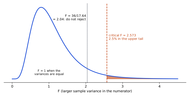
The F-distribution is right-skewed, bounded below by zero and defined by two degrees of freedom (numerator , denominator ). when the sample variances are equal. Putting the larger variance in the numerator means only the upper critical value matters (with in that tail for a two-tailed test).
- (the variances are not different) vs. .
- If the F-statistic exceeds the critical F-value, reject and conclude that the variances are significantly different. Example. With () and (), . The critical value with 2.5% in the upper tail is 2.573, so the null is not rejected.
Test of a correlation coefficient
The correlation coefficient (the Pearson correlation) gauges how strong a linear relationship is and lies between −1 (perfect negative) and +1 (perfect positive); zero means no linear relationship. vs. . The statistic needs only the sample correlation and the sample size ; it follows a t-distribution with degrees of freedom. It grows with and with , so a modest correlation can be significant in a large sample: gives with but only with .
Example. With and , . This exceeds , so is rejected.
When a table is given, select the row for df and the column for the stated (two-tailed) significance level. The null is rejected at a given level only if exceeds that column's value.
p-values and p-hacking
The p-value is the smallest significance level at which the null can be rejected (the probability, if is true, of a statistic at least as extreme as the one observed). Reject when p-value < . p-hacking is manipulating data or the testing process to manufacture a statistically significant result, e.g.:
- testing only the best periods, or deleting inconvenient observations as "outliers";
- data mining: running many tests until one rejects the null (with , about 1 in 20 tests of true nulls rejects by chance);
- using smoothed (e.g., appraisal-based) data to understate risk.
Because it produces rejections of nulls that are actually true, p-hacking raises the frequency of Type I errors (false positives). It is not the same as legitimately choosing a significance level or seeking a more powerful test.
Common exam traps
- df: correlation test ; single mean, paired test and single variance ; difference in means (pooled, equal population variances assumed); F-test .
- Chi-square tests one variance; F tests two variances; t tests means and correlations.
- The same subjects measured twice call for a paired comparisons test rather than a difference-in-means test.
- Rejecting in an F-test means concluding the variances are different.
Exam shortcuts
- Choose the test from what is tested: a mean uses t when the population variance is unknown (z when it is known, or as a large-sample approximation), a test that a correlation is zero uses t when both variables are normally distributed, one variance uses chi-square, and two variances use F.
- With the larger variance in the numerator of the F-statistic, only the upper critical value is needed.
- When a p-value is given, reject if it is below ; no critical value is needed.
Bottom line
- Independent samples with equal variances use the pooled difference-in-means t-test with df; the same subjects measured twice use the paired comparisons test with df.
- A single variance is tested with and df; the chi-square distribution is right-skewed and bounded below by zero.
- Two variances are tested with and , df.
- A correlation is tested with and df; the statistic rises with and with .
- The p-value is the smallest significance level at which can be rejected.
- p-hacking raises the frequency of Type I errors.
Quick check
An analyst tests whether a currency strategy's mean daily return is zero and obtains a p-value of 0.021. Which conclusion is most accurate?
Show answer and explanation
Correct answer: C
The p-value is the smallest significance level at which the null hypothesis can be rejected. The null is rejected whenever the chosen α exceeds the p-value, so here it is rejected at 5% or at 2.5% but not at 1%.
Why the other options are wrong
- A. At 1%, the p-value of 0.021 is above α = 0.01, so the null is not rejected.
- B. The p-value is computed assuming the null is true: it is the probability, under , of a test statistic at least as extreme as the one observed. It does not measure the probability that itself is true.
Key takeaway Reject when the p-value is below α. A p-value of 0.021 rejects at 5% but not at 1%.
Module 7.4
Nonparametric Hypothesis Tests
LOS 7.c — Parametric vs. nonparametric tests
When is a test nonparametric?
| Parametric test | Nonparametric test | |
|---|---|---|
| What is tested | A parameter of a distribution (mean, variance, correlation) | Something that is not a parameter (ranks, counts in categories), or a parameter when assumptions fail |
| Assumptions | Specific distribution (e.g., normal population) | Few or no distributional assumptions |
| Typical data | Values measured on a scale | Ranks or categorical data |
| Accuracy | Tends to be more accurate when its assumptions hold | More flexible, but tends to be less accurate when the parametric assumptions hold |
Use a nonparametric test when (1) the data are ranks or categories, (2) the distributional assumptions of a parametric test do not hold (e.g., a small sample from a clearly non-normal population, so the CLT cannot be relied on), or (3) the question is not about a parameter at all, for example whether two sets of ranks are related or whether a set of observations is consistent with a particular distribution.
Spearman rank correlation test
The Spearman rank correlation measures the strength of a monotonic relation between two sets of ranks (e.g., a fund's performance rank this year vs. next year). With integer ranks and = difference between the two ranks of item :
Key concept
Example. For six funds with rank differences of 1, −1, 0, 2, −1 and −1, and .
Significance is tested with the same statistic as a Pearson correlation, , which for large samples () follows a t-distribution with df. A test of whether performance ranks persist is therefore a nonparametric test.
Test of independence using a contingency table
A contingency table counts observations classified by two categorical characteristics (e.g., issuer sector × credit-rating change). The chi-square test of independence asks whether the two characteristics are related.
- : the two characteristics are independent. : they are not independent.
- Expected frequency of cell if independent. Under independence an observation's row says nothing about its column, so each row total is split across the columns in the same proportions as the column totals:
- Test statistic (sum over all cells of squared deviations, each scaled by the expected count):
- Reject independence if exceeds the critical chi-square value (right tail only).
- The standardized residual (Pearson residual) of a cell is ; its square is that cell's contribution to .
- Exam convention: each standardized residual is approximately standard normal, and cells with values beyond ±2 are flagged as contributing significantly to the lack of independence.
- Current practice: because the row and column totals are estimated from the data, the raw residual has a variance below 1, so ±2 works as a screening rule of thumb. The adjusted residual, which divides by , is the one that is approximately standard normal.
Example. A sample of 220 bonds is classified by issuer size and rating action over a year:
| Issuer size | Upgraded | Unchanged | Downgraded | Total |
|---|---|---|---|---|
| Small | 42 | 38 | 20 | 100 |
| Large | 18 | 62 | 40 | 120 |
| Total | 60 | 100 | 60 | 220 |
Expected (small, upgraded) . Summing over the six cells gives with df. The 5% critical value is 5.991 (1%: 9.210), so independence is rejected. The standardized residual for (small, upgraded) is : by the ±2 rule of thumb, small issuers were upgraded notably more often than independence implies.
Common exam traps
- The df for a contingency table are ; and are common errors. Count only the category rows and columns and leave out the "Total" row and column. For the 2 × 3 bond table the df are 2; gives 3 and gives 6.
- Expected counts come from the row and column totals rather than from the observed cell.
- The statistic divides each squared deviation by the expected count; the plain sum of deviations is always zero.
- Rank data (e.g., performance rankings) call for a nonparametric Spearman test; category counts call for a chi-square test on a contingency table.
- Standardized residuals are screened against the ±2 rule of thumb cell by cell, while the overall statistic is compared with a chi-square critical value.
Exam shortcuts
- Rank data point to the Spearman test; category counts point to a chi-square test on a contingency table.
- Contingency table df are , counting only category rows and columns and leaving out the totals.
Bottom line
- A nonparametric test is used for ranks or categories, when the assumptions of a parametric test do not hold, or when the question is not about a parameter.
- The Spearman rank correlation is , tested in large samples () with the same t-statistic as a Pearson correlation.
- In a chi-square test of independence the expected count is row total × column total ÷ total, with df, and only the right tail is used.
- A standardized residual is , and cells beyond ±2 are flagged by the rule of thumb.
Quick check
A credit researcher compiles the following default data for bond issuers in three sectors:
| Sector | No default | Technical default | Actual default | Total |
|---|---|---|---|---|
| Energy | 94 | 16 | 15 | 125 |
| Healthcare | 108 | 9 | 13 | 130 |
| Utilities | 126 | 8 | 16 | 150 |
| Total | 328 | 33 | 44 | 405 |
Assuming sector and default status are independent, the expected number of energy issuers in technical default is closest to:
Show answer and explanation
Correct answer: A
Under independence, the expected count for a cell is (row total × column total) / total number of observations. For energy issuers in technical default, use the Energy row total (125) and the Technical default column total (33).
Why the other options are wrong
- B. About 14 (13.6) uses the Actual default column total (44) instead of the Technical default column total: .
- C. 16 is the observed number of energy issuers in technical default; the question asks for the count expected under independence.
Key takeaway Expected count = row total × column total / grand total.
Practice Questions
A multi-asset portfolio is worth €40 million, and its daily returns have a standard deviation of 1.2%. Using the parametric method and assuming a daily mean return of zero, the portfolio's daily 5% value at risk (VaR) is closest to:
Show answer and explanation
Correct answer: A
Parametric value at risk assumes normally distributed returns. With a zero mean, the 5% VaR is the loss that sits 1.645 standard deviations below the mean, with the whole 5% in the left tail. It means there is a 5% probability of losing that amount or more on any given day.
One-tailed critical value for 5%: (exact 1.6449; many texts round to 1.65).
(With 1.65 the result is €792,000 — still closest to €0.79 million.)
Why the other options are wrong
- B. €0.94 million uses 1.96, the two-tailed 5% value (2.5% in each tail). VaR is one-tailed, so the full 5% belongs in a single tail (z = 1.645).
- C. €1.12 million uses 2.33, the one-tailed critical value for 1%, which gives the 1% VaR.
Key takeaway VaR puts the whole in one tail: 1.28 for 10%, 1.645 for 5% and 2.33 for 1%. It is the minimum loss at that probability; larger losses remain possible.
This reading has 67 questions in the full bank. Practice all of them.
Key Takeaways
- Dividing the population into groups first and then sampling randomly within every group is stratified random sampling.
- VaR puts the whole in one tail: 1.28 for 10%, 1.645 for 5% and 2.33 for 1%. It is the minimum loss at that probability; larger losses remain possible.
- With fixed, a lower means a higher and a lower power.
- Reject when the p-value is below α. A p-value of 0.021 rejects at 5% but not at 1%.
- Expected count = row total × column total / grand total.