Quantitative Methods · Reading 6
Lognormal Distribution
CFA Level I · Quantitative Methods · Reading 6: Statistical Distributions for Financial Asset Prices and Returns · about 1 h 2 min
What you'll learn
- LOS 6.a Compute and interpret the unconditional mean, variance, standard deviation and covariance of random variables, including from scenario and joint probability tables.
- LOS 6.b Describe the shape, principal moments and typical financial uses of the discrete uniform, binomial, Poisson, continuous uniform, normal, lognormal and logistic distributions.
- LOS 6.c Compute and interpret conditional expectations, variances and covariances, including from joint probability tables and probability trees.
- LOS 6.d Use Bayes' formula to update a prior probability into a posterior probability when new information arrives.
Module 6.1
Probability Distributions and Expected Values
This reading describes random variables through their probability distributions and summarizes them with the expected value, variance and covariance. It then matches the common discrete and continuous distributions to the financial quantities they model, and shows how conditional expectations and Bayes' formula update a forecast when new information arrives.
LOS 6.a — Unconditional mean, variance and covariance of a random variable
Random variables: discrete vs. continuous
A random variable is a quantity whose value is not known until an outcome is observed. It is also called a stochastic variable.
| Feature | Discrete random variable | Continuous random variable |
|---|---|---|
| Possible values | A countable set (e.g., the number of issuers in a 50-bond portfolio downgraded this year) | Infinitely many values inside a range (e.g., tomorrow's percentage change in the gold price) |
| Probability function | Probability mass function (PMF): can be positive | Probability density function (PDF): for every single point |
| Probabilities are assigned to | Individual outcomes | Intervals, e.g. |
| Can outcomes be negative? | Yes, if the countable set includes negatives | Yes, or the range may be restricted to positive values |
A probability distribution lists the probabilities of all possible outcomes of a random variable, and these probabilities sum to 1. A probability function gives the probability that X equals a particular value. For a discrete variable, for a value that cannot occur and for one that can.
Whether a variable is discrete does not depend on its outcomes being equally likely (the uniform case) or positive. Prices quoted in cents are technically discrete. Because there are so many possible values, analysts usually treat them as continuous and speak of the probability of a range of price changes.
What makes a valid probability function
A function qualifies as a probability function only if both conditions hold:
Key concept
- for every possible outcome ;
- over all possible outcomes.
A list such as 0.50, 0.40, 0.20, −0.10 sums to one but fails condition 1. Five values of 0.25 each pass condition 1 but sum to 1.25, so they fail condition 2.
For a continuous variable, a single point carries no probability, so including or excluding the endpoints does not change the probability of an interval: . The height of the PDF at a point is a density. A probability is the area under the PDF over an interval.
Cumulative distribution function (CDF)
The cumulative distribution function (CDF), also called the distribution function, gives the probability that X takes a value less than or equal to x:
For a discrete variable, is the sum of the probabilities of all outcomes up to and including x. For the standard normal distribution (Module 6.2), : the area under the PDF to the left of −1 equals the height of the CDF at −1.
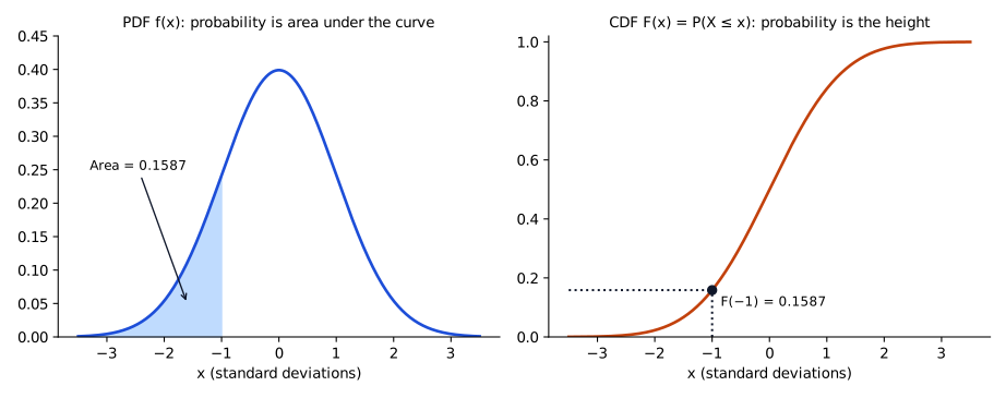
Example. A fund's quarterly return is continuous on with . Then .
Unconditional expected value (mean)
The unconditional mean (also the unconditional expectation or expected value) weights each outcome by its probability:
The weights are the probabilities, and they must sum to 1, so a probability that is not stated can be found as 1 minus the sum of the others. A simple average of the outcomes weights each by , so it is the expected value when every outcome is equally likely; with unequal probabilities it generally gives a different answer. The sample mean of Reading 5 summarizes returns already observed (an ex post measure). An expected value weights possible future outcomes by their probabilities, so it is a forecast (an ex ante measure).
Unconditional variance and standard deviation
The unconditional variance is the probability-weighted squared spread around the expected value, and the unconditional standard deviation is its square root:
Key concept
Variance is in squared units (e.g., %²), so the standard deviation (back in % units) is the figure compared with returns. An equivalent shortcut is .
Unconditional covariance
Unconditional covariance shows the direction of the linear relationship between two random variables, that is, whether they tend to be above or below their own means at the same time. Its strength is read from the correlation (last point below). The covariance is computed as:
The shortcut form is .
- Positive covariance: the variables tend to move in the same direction; negative: opposite directions.
- For scenario (state) tables, is simply the probability of the state. In a joint probability table, cells with zero probability contribute nothing.
- Units are the product of the two variables' units (e.g., %² or decimal²), so the size is hard to interpret. Dividing by the two standard deviations gives the unit-free correlation: , which always lies between −1 and +1.
| Measure | Formula core | Units | Range |
|---|---|---|---|
| Variance | squared units | ||
| Covariance | product of units | any sign, unbounded | |
| Correlation | none | to |
Worked example
| State | Probability | Return on P | Return on Q |
|---|---|---|---|
| Expansion | 0.20 | 15% | 4% |
| Normal | 0.50 | 8% | 7% |
| Downturn | 0.30 | −2% | 2% |
- ; .
- (%²), so .
- (%²), so .
- (%²).
- .
Calculator. The BA II Plus DATA/STAT worksheet computes a probability-weighted mean when each outcome is entered with a frequency proportional to its probability (e.g., 20, 50 and 30). The mean is and the population standard deviation is .
Common exam traps
- Averaging outcomes equally instead of weighting by probabilities. For portfolio P in the worked example, the simple average is , against an expected return of 6.4%.
- Forgetting the square root: reporting the variance when the standard deviation is asked, or mixing decimals (0.0035) with percent-squared (35.04). For portfolio P in the worked example, the variance is 37.24 (%²) and the standard deviation is 6.10%.
- Using absolute deviations instead of squared deviations, which gives a different measure from the variance and standard deviation.
- Computing covariance without the probabilities, or dividing an unweighted sum of cross-products by the number of states.
- Confusing covariance with correlation; the answer to "covariance" carries squared units and is not bounded by ±1.
- Believing a continuous variable has a positive probability at a single point, or that the PDF height is a probability.
- Reading a CDF value as the probability of that single outcome, or leaving the outcome itself out of .
Exam shortcuts
- When the outcomes listed are mutually exclusive and exhaustive and one probability is missing, it equals 1 minus the sum of the others.
- Variance can be found as , which avoids computing each deviation.
- For a continuous variable, including or excluding the endpoints does not change the probability of an interval.
Bottom line
- A discrete random variable has a probability mass function with positive probabilities at individual outcomes; a continuous variable has a density, zero probability at any single point and probabilities assigned to intervals.
- A probability function is valid only if every lies between 0 and 1 and the probabilities sum to 1.
- The CDF is , and .
- Expected value is ; variance is in squared units, and the standard deviation is its square root.
- Covariance shows only the direction of co-movement; correlation is unit-free and lies between −1 and +1.
Quick check
A random variable X can take only the values 0, 1, 2 and 3. Which of the following proposed functions is a valid probability function for X?
Show answer and explanation
Correct answer: C
A probability function must satisfy two conditions: every probability lies between 0 and 1 inclusive, and the probabilities over all possible outcomes add up to exactly 1. Only meets both: it gives 0.1, 0.2, 0.3 and 0.4, each within [0, 1], summing to 1.0.
- Set with : sum , but , so it fails condition 1.
- Constant : each value is within [0, 1], but the sum is , so it fails condition 2.
- : ; all in [0, 1] and , so it is valid.
Why the other options are wrong
- A. The probabilities sum to one, but a negative probability is impossible; satisfying only the 'sum to one' condition is not enough.
- B. Each probability is between 0 and 1, but together they sum to 1.20. A probability function must exhaust exactly 100% of the probability; an equal-probability function over four outcomes would need 0.25 each.
Key takeaway Check both conditions every time: for each x, and .
Module 6.2
Discrete and Continuous Probability Distributions
LOS 6.b — Moments and uses of the key distributions in finance
The four principal moments
| Moment | What it describes | Benchmark (normal distribution) |
|---|---|---|
| 1. Mean | Central location | — |
| 2. Variance | Dispersion around the mean | — |
| 3. Skewness | Asymmetry; positive = long right tail | 0 (symmetric) |
| 4. Kurtosis | Weight of the tails relative to the center | 3 (excess kurtosis = kurtosis − 3 = 0) |
The most useful features of each distribution are what it models and its shape: bounded or unbounded, symmetric or skewed, thin or fat tails. The moment formulas below are for reference.
| Distribution | Mean | Variance | Skewness | Excess kurtosis |
|---|---|---|---|---|
| Discrete uniform ( outcomes, to ) | 0 | |||
| Binomial | ||||
| Poisson | ||||
| Continuous uniform | 0 | −1.2 | ||
| Normal | 0 | 0 | ||
| Lognormal | ||||
| Logistic | 0 | 1.2 |
Discrete distributions
Discrete uniform. A finite set of outcomes, each with probability (e.g., the integers 1 to 8, each with probability 0.125); the probability of outcomes in a range is , and the CDF at the th outcome is . For a discrete uniform variable on the consecutive integers : mean and variance . For a general equally likely set (e.g., ), compute the arithmetic mean and the population variance directly: here the mean is 3 and the variance is . The consecutive-integer formula would wrongly give 2.
Binomial. Counts the number of successes in a fixed number of independent trials, each with the same success probability and only two possible results (success/failure). A binomial variable with a single trial is a Bernoulli distribution.
Key concept
Example. 16 independent new-issue auctions, each with a 0.75 chance of being fully covered: expected fully covered auctions ; variance . The expected number of successes need not be a possible outcome (10 trials with give 4.3); it is the average number of successes over many repetitions.
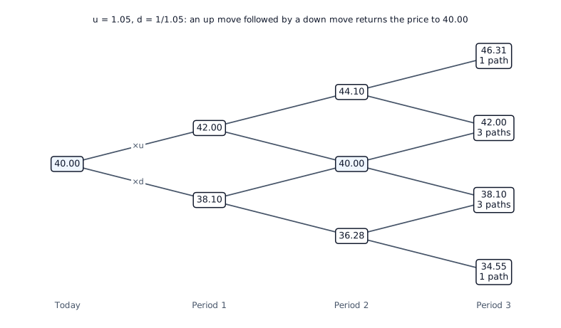
Binomial models are also used for asset prices: at each step the price is multiplied by an up factor or a down factor , so after up moves and down moves the price is . The possible paths are drawn as a probability tree (or decision tree). With and , a price of 40 after one up and one down move returns to 40, whatever the order.
Poisson. Counts how many times an event occurs in a fixed interval when events arrive independently at a known, constant average rate . It is the usual model for rare events such as defaults per year, trading halts per month or operational losses per quarter.
Example. With outages per year, , so the probability of at least one outage is . For a pool of independent credits each with default probability , . The Poisson is the limit of a binomial as and with fixed.
Continuous distributions
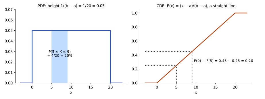
Continuous uniform on : every equal-width sub-interval is equally likely, so the CDF rises in a straight line, for .
Key concept
Skew 0, kurtosis 1.8 (excess −1.2). Used to generate random draws for Monte Carlo simulation. Example. Uniform on [0, 20]: .
Normal (also called the Gaussian distribution), : symmetric bell curve, fully described by its mean and variance, or equivalently its mean and standard deviation (skew 0, excess kurtosis 0). About 68% of outcomes lie within ±1σ and about 95% within ±2σ. Sums of many independent variables tend toward normality, and a binomial converges to a normal as grows. It is unbounded in both directions, so it can produce negative values. The normal with mean 0 and variance 1, , is the standard normal distribution; its horizontal axis measures standard deviations from the mean.
Example. Annual returns are normal with a mean of 7% and a standard deviation of 15%. About 68% of years should fall between and , and about 95% between −23% and 37%. A −23% return lies standard deviations from the mean. The curve is symmetric, so the 5% of years outside split evenly: about 2.5% of years should lose more than 23%. Subtracting the two bands gives the share between them: about of outcomes lie between one and two standard deviations below the mean, and the same share lies between one and two standard deviations above it.
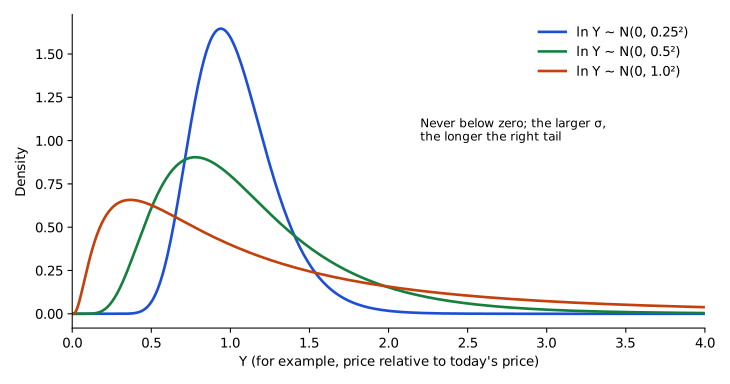
Lognormal. is lognormal when is normal; equivalently with normal.
- Because for any , the lognormal is bounded below by zero and never takes a negative value.
- It is positively (right) skewed, with a long right tail.
- That makes it well suited to modeling asset prices. A price following a lognormal cannot fall below zero, so the implied return can never be worse than −100%. A normal price model, by contrast, would allow negative prices (returns below −100%), which is impossible for a limited-liability asset.
- If continuously compounded price returns (no distributions paid) are normally distributed, then prices are lognormal, because with normal. Over several periods, is the sum of the one-period log returns (Reading 1), and sums of many independent returns tend toward a normal distribution. A lognormal price model therefore fits well even when single-period returns are not exactly normal.
- Its two parameters are the mean and SD of , called the location parameter and the scale parameter. They are not the mean and SD of itself: the mean of is .
- Prices can be projected with a geometric Brownian motion model. Here is the expected (arithmetic) growth rate of the price, not the location parameter of used above, and is the drift term: . Example. , , , : , so .
- Exam convention: the price from the drift-term formula is the expected price in years. Current practice: with as the expected growth rate, that figure is the median of the lognormal price distribution; the mean price is (here ), which is higher because of the right skew.
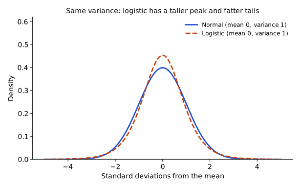
Logistic. Bell-shaped and symmetric like the normal (skew 0), but with fatter tails. Its excess kurtosis is +1.2, so extreme outcomes are more likely than under a normal with the same variance. The variance is for scale parameter . The logistic distribution is used in logistic regression, where the dependent variable is binary (0/1), and in machine learning.
Matching the distribution to the problem
| Situation | Distribution |
|---|---|
| Number of successes in a fixed number of independent yes/no trials | Binomial |
| Count of rare events in an interval at a constant rate | Poisson |
| Equally likely finite outcomes | Discrete uniform |
| Random draws for simulation over a range | Continuous uniform |
| Returns, test statistics, sums of many variables | Normal |
| Asset prices (non-negative, right-skewed) | Lognormal |
| Binary-outcome regression; symmetric but fat-tailed data | Logistic |
Common exam traps
- Calling the Poisson a "timing" or "waiting-time" distribution: it models the count of events in an interval.
- Thinking a lognormal is negatively skewed or symmetric; it is positively skewed and bounded at zero.
- Reversing the log relation: if is lognormal then is normal (not lognormal); if is normal then is lognormal.
- Saying a normal is appropriate for prices "because it only lets prices fall to zero". A normal is unbounded and allows negative prices.
- Attributing skewness to the logistic distribution: its skew is zero, and it differs from the normal in kurtosis (fatter tails).
- Using the binomial when the number of trials is not fixed or the success probability changes from trial to trial.
Exam shortcuts
- Identify the distribution from the wording: successes in a fixed number of trials is binomial, a count of events in an interval is Poisson, random draws for simulation are continuous uniform, and asset prices are lognormal.
- Normal bands: about 68% of outcomes lie within ±1σ and 95% within ±2σ, so about 2.5% lie beyond 2σ on each side and about 13.5% lie between 1σ and 2σ on each side.
- For a Poisson variable, the probability of at least one event is .
Bottom line
- A binomial variable counts successes in independent trials with a constant : and ; a single trial is a Bernoulli distribution.
- A Poisson variable counts events in an interval at a constant rate , and its mean and variance both equal .
- For a continuous uniform variable on , .
- The normal distribution is symmetric, fully described by its mean and variance, and unbounded in both directions.
- If is normal, is lognormal: bounded below by zero and positively skewed, which suits asset prices.
- The logistic distribution is symmetric like the normal but has fatter tails (excess kurtosis +1.2).
Quick check
Each week, the fixed-income desk at Corrib Securities submits competitive bids in 25 separate government bond auctions. The desk's chance of winning an allocation is 0.36 in every auction, and the result of one auction does not affect any other. For the number of auctions the desk wins in a week, the expected value and the variance are, respectively:
Show answer and explanation
Correct answer: C
The number of wins is a binomial random variable: there is a fixed number of independent trials (25 auctions), each with only two outcomes (win or lose) and the same probability of success (). Its mean is and its variance is .
(The standard deviation would be .) As with any discrete count, the mean of 9.0 is the long-run average number of wins per week, not a guaranteed result.
Why the other options are wrong
- A. 16.0 uses the probability of losing an auction, , so it is the expected number of losses. The variance of 5.76 is right, because is the same whichever outcome is called a success.
- B. The mean of 9.0 is right, but 2.40 is the standard deviation, , which is the square root of the variance.
Key takeaway Binomial: and . Define "success" as the outcome being counted, and do not stop at the standard deviation when the variance is asked.
Module 6.3
Conditional Expectations and Bayesian Updating
LOS 6.c — Joint distributions, conditional expectations, variances and covariances
Joint and marginal probabilities
A joint probability distribution gives the probability of every combination of outcomes of two or more variables; for two variables it is bivariate. For discrete variables it is often shown as a contingency table. Row and column totals are the marginal distributions.
For two variables in general, the joint cumulative distribution function gives the probability that both variables are at or below given values: . A bivariate distribution is described by each variable's mean and variance plus how they move together (their covariance or correlation).
| 400 listed firms | Technology | Non-technology | Total |
|---|---|---|---|
| Return > 10% | 64 | 56 | 120 |
| Return ≤ 10% | 96 | 184 | 280 |
| Total | 160 | 240 | 400 |
- Marginal: ; .
- Joint: .
- Conditional: , using only the technology column.
Conditional mean, variance and covariance
A conditional expectation is the expected value of given that condition holds, read "the expected value of X given S". A forecast revised for new information is a conditional expectation; for example, "if the merger is approved, my EPS estimate rises to $4.20".
The conditional variance measures dispersion around the conditional mean rather than the unconditional mean :
The conditional covariance is defined the same way for two variables, using conditional probabilities and conditional means. It is a different concept from the conditional variance of one variable.
A conditional distribution describes one variable after the other variables in a joint distribution are restricted to certain values. Conditioning changes the relevant probability distribution, so it can change both the expected value and the variance.
| Concept | Probabilities used | Deviations measured from |
|---|---|---|
| Unconditional mean/variance | over all outcomes | |
| Conditional mean/variance | over outcomes consistent with | |
| Joint probability | — (not an expectation) |
Probability trees
A tree shows sequential outcomes; the probability of a full path is the product of the branch probabilities along it. The unconditional expected value weights every end node by its path probability, the product of the branch probabilities along that path. Imposing a condition (for instance, "the price fell in period 1") prunes the tree. Only branches that start from the observed node remain, and their branch probabilities become the conditional probabilities.
Example. A share at 50 moves up 10% with probability 0.6 or down 10% with probability 0.4 in each of two periods (independent moves).
- End prices: 60.50 (prob. 0.36), 49.50 (prob. 0.48 via two paths), 40.50 (prob. 0.16). Unconditional .
- Given (a fall in period 1): ; , so the conditional SD is 4.41.
- Given : . Weighting the two conditional expectations by their branch probabilities gives back the unconditional value, .
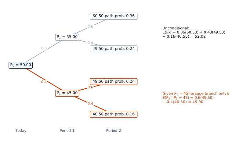
A common error is to weight the remaining outcomes by their joint (path) probabilities, e.g. , which gives 18.36. That figure is rather than the conditional expectation.
LOS 6.d — Updating probabilities with Bayes' formula
Bayes' formula revises a prior probability (also called an a priori probability) of an event into a posterior probability after new information is observed. It follows from the multiplication rule, : writing the joint probability two ways gives , and dividing by gives
Key concept
The denominator is the unconditional probability of the information: the sum of its joint probabilities with each state.
The formula can be checked against the 400-firm table in LOS 6.c. Counting directly, 64 of the 120 firms that returned more than 10% are technology firms, so . Bayes' formula reaches the same figure from the reverse conditional probability: .
Applying Bayes' formula:
- Write down the prior and its complement .
- Write down the likelihoods and ; take complements if the information is a "does not happen" event.
- Multiply to get the joint probabilities of with each state.
- Add the joint probabilities to get .
- Posterior = the joint probability for the state of interest ÷ .
Example. Of the fund managers in a database, 30% are skilled. A skilled manager beats the benchmark in a given year with probability 0.75; an unskilled one with probability 0.40. A manager beat the benchmark. What is the probability that she is skilled?
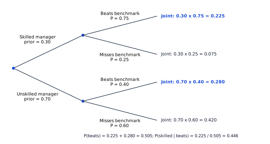
The evidence raises the probability from the 30% prior to about 45%, but because unskilled managers are the majority, a single good year is far from proof of skill.
Common exam traps (LOS 6.c and 6.d)
- Reporting the joint probability (step 3) as the answer instead of dividing by . In the fund manager example this gives 0.225 instead of 0.446.
- Reporting (step 4), the unconditional probability of the information, instead of the posterior. In the same example this gives 0.505.
- Confusing with ; they are generally very different.
- Comparing likelihoods only, , which ignores the priors. There it gives .
- Forgetting to use complements when the information is that something did not happen.
- In trees, using joint path probabilities for a conditional expectation, or averaging all end nodes equally.
- Measuring conditional variance around the unconditional mean.
Exam shortcuts
- For Bayes' formula, write one row per state with prior × likelihood, add the rows to get , and divide the row for the state of interest by that total.
- Check a conditional expectation answer: the conditional expectations weighted by their branch probabilities must give back the unconditional expectation.
Bottom line
- A joint probability is , marginal probabilities are the row and column totals, and a conditional probability uses only the outcomes consistent with the condition.
- The conditional expectation is , and the conditional variance is measured around .
- In a probability tree a path probability is the product of its branch probabilities.
- Bayes' formula is , where adds the joint probabilities of the information with every state.
- and are generally different, and the posterior still depends on the prior.
Quick check
A high-yield portfolio holds 40% BB-rated bonds and 60% B-rated bonds. Historically, 10% of BB-rated bonds and 30% of B-rated bonds default within five years. If a bond chosen at random from the portfolio defaults within five years, the probability that it was BB-rated is closest to:
Show answer and explanation
Correct answer: B
This is a Bayesian update: the prior probability that a bond is BB-rated (0.40) is revised using the information that the bond defaulted. The posterior is the joint probability of 'BB and default' divided by the unconditional probability of default.
Why the other options are wrong
- A. 0.100 is , the likelihood. The question asks for the reverse conditional probability, the posterior .
- C. 0.333 is the ratio of the two default rates (); it ignores the portfolio weights (priors) and the unconditional probability of default.
Key takeaway . Build the joint probabilities, add them for the denominator, then divide.
Practice Questions
A consultant at Northgate Partners has estimated the scenario returns shown in the table below. The standard deviation of returns on Fund Alder is closest to:
| Scenario | Probability | Return on Fund Alder | Return on Fund Birch |
|---|---|---|---|
| Boom | 20% | 19% | 12% |
| Expansion | 25% | 15% | 11% |
| Stagnation | 35% | 9% | 10% |
| Contraction | 20% | 1% | 8% |
Show answer and explanation
Correct answer: B
The standard deviation of Fund Alder is the square root of the probability-weighted average squared deviation of Alder's scenario returns from Alder's expected return. Fund Birch's column is irrelevant to this question.
1. Expected return on Alder
2. Variance (percent units)
(in decimals, 0.003819)
3. Standard deviation
Why the other options are wrong
- A. 1.34% is the standard deviation of Fund Birch, computed from the wrong column (variance 1.7875 %²).
- C. 6.78% ignores the probabilities and treats the four scenarios as equally likely (mean 11%, variance 46 %²).
Key takeaway Read the column carefully in two-asset tables, and weight squared deviations by the scenario probabilities.
A commodity desk simulates thousands of possible copper price paths and wants to be certain that no simulated price is ever negative. Which distribution for the price level is best suited to this goal?
Show answer and explanation
Correct answer: C
The lognormal distribution is bounded below by zero, so it can never generate a negative price, which is why it is the usual choice for modeling asset price levels. Both the normal and the logistic distributions extend to minus infinity.
Why the other options are wrong
- A. A normal distribution is unbounded below, so with enough simulated paths some prices would turn negative; it is unsuitable for modeling price levels directly.
- B. A logistic distribution is also symmetric and unbounded, allowing negative as well as positive values (and its fat tails make extreme negative draws even more likely than under a normal).
Key takeaway When simulated prices must never be negative, model the price level as lognormal.
This reading has 46 questions in the full bank. Practice all of them.
Key Takeaways
- Check both conditions every time: for each x, and .
- Read the column carefully in two-asset tables, and weight squared deviations by the scenario probabilities.
- Binomial: and . Define "success" as the outcome being counted, and do not stop at the standard deviation when the variance is asked.
- When simulated prices must never be negative, model the price level as lognormal.
- . Build the joint probabilities, add them for the denominator, then divide.