Quantitative Methods · Reading 5
Skewness and Kurtosis
CFA Level I · Quantitative Methods · Reading 5: Statistical Characteristics of Asset Returns · about 58 min
What you'll learn
- LOS 5.a Calculate, interpret and evaluate measures of dispersion: range, mean absolute deviation, variance and standard deviation (population and sample).
- LOS 5.b Describe, interpret and evaluate skewness and kurtosis and their effect on the mean, median, mode and tail risk of a return distribution.
- LOS 5.c Calculate, interpret and evaluate covariance and correlation, including the limits of correlation (linear only, no causation, spurious correlation) and the use of scatter plots.
- LOS 5.d Calculate, interpret and evaluate semivariance, target downside deviation and the coefficient of variation as measures of downside and relative risk.
Module 5.1
Measures of Central Tendency
This reading summarizes a return distribution with measures of central tendency and location (mean, median, mode, trimmed and winsorized means, quantiles) and of dispersion (range, mean absolute deviation, variance and standard deviation), and it interprets skewness and kurtosis. It then calculates the covariance and correlation of two variables and measures downside risk and relative dispersion with the target downside deviation and the coefficient of variation.
LOS 5.a — Central tendency and location
A measure of central tendency summarizes where the "center" of a dataset lies, so a single number can stand for the typical or expected value. A measure of location (quantiles) describes where a given observation sits within the distribution.
Population vs. sample
A population is every element of interest (e.g., all monthly returns a fund has ever earned). A sample is a subset of it (e.g., the last 36 months). Sample statistics are used to make inferences about population parameters. Of all the measures of central tendency, analysts rely on the arithmetic mean most often.
The three classic measures
Key concept
| Measure | Definition | Sensitive to outliers? | Notes |
|---|---|---|---|
| Arithmetic mean | Sum of the observations divided by their number (every value weighted equally) | Yes; one extreme value can move it a lot | The sample mean is an arithmetic mean |
| Median | Middle value of the data sorted in order; with an even count, the average of the two middle values | No; it is a robust estimator (reliable with outliers or when the data come from a different distribution than assumed) | Half of the observations lie above it, half below |
| Mode | Most frequently occurring value | No | A dataset can have one mode, two (bimodal), several, or none |
For continuous data such as returns, exact repeats are rare, so outcomes are grouped into intervals and the modal interval, the interval containing the most observations, is reported.
The geometric mean measures the compound growth rate of returns. Like the arithmetic mean, it uses every observation, so it is also pulled by extreme values.
Example. Six monthly returns: 4%, −1%, 7%, 4%, 2%, 20%.
- Mean .
- Sorted: −1, 2, 4, 4, 7, 20, so the median .
- Mode (appears twice).
The single 20% month pulls the mean above both the median and the mode. Replace 20% with 9% and the mean falls to 4.17%, while the median and mode stay at 4%.
Dealing with outliers
Outliers are unusually large or small observations. They can come from measurement, data entry or sampling errors, or simply from the real variability of the data. If they are errors, they distort the mean. If the data are measured correctly, keeping every value may be best, because deleting genuine observations throws away information about the distribution.
- Trimmed mean: drop a set percentage of the observations at the extremes, split equally between the two ends, then average what remains. Trimming identifies the outliers objectively but may remove useful information. A 4% trimmed mean drops the lowest 2% and the highest 2%. The denominator is the number of observations remaining.
- Winsorized mean: keep every observation but replace the extremes with percentile values. For a 96% winsorized mean, values below the 2nd percentile are set equal to the 2nd percentile and values above the 98th percentile are set equal to the 98th percentile; then take the mean of all values.
Key concept
| Trimmed mean | Winsorized mean | |
|---|---|---|
| Extreme values | Removed | Replaced by percentile values |
| Number of values averaged | Fewer than | All |
| Information kept | Less | More |
With only a small number of outliers, the winsorized mean is a better measure of the center than either the arithmetic mean or a trimmed mean. Both adjustments move the estimate away from the side where the extremes lie: a few huge positive values make the trimmed/winsorized mean lower than the arithmetic mean; a few huge negative values make it higher.
Quantiles
A quantile is a cut-off value: a given share of the observations lies at or below it. The median is the 50th percentile, which is also the second quartile and the fifth decile.
Key concept
| Quantile | Divides the data into | Example |
|---|---|---|
| Quartile | 4 parts | 3rd quartile = 75th percentile |
| Quintile | 5 parts | 1st quintile = 20th percentile |
| Decile | 10 parts | 9th decile = 90th percentile |
| Percentile | 100 parts | An observation at the 70th percentile has 70% of the observations below it |
Because each quantile is named by the share of observations at or below it, the positions always run in the same order: first decile (10th percentile), first quintile (20th), first quartile (25th), median (50th). A lower position can equal but never exceed a higher one.
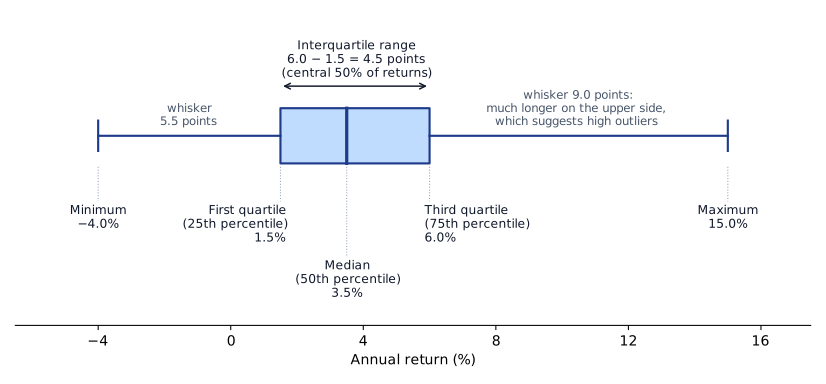
The interquartile range (IQR) runs from the first quartile (25th percentile) to the third quartile (75th percentile), so its width is . It contains the central 50% of the data.
A box and whisker plot draws a box that spans the interquartile range, a line inside the box marks the median, and the whiskers extend to the smallest and largest observations (the full range). A whisker much longer on one side hints at outliers on that side.
Stationarity
Statistical inference works best when data are stationary: the mean and variance of the underlying distribution do not change over time. If they do change, the series is nonstationary and forecasts or tests based on it are less reliable. Price or index levels that trend upward are typically nonstationary; their periodic percentage changes are much more likely to be stationary.
Common exam traps
- Calling the middle value of ordered data the mean. It is the median; with an even count, average the two middle values.
- Assuming that a value equal to the median also equals the mean. The two may be close without being equal, so compute the mean before choosing.
- Expecting the median to move when only the largest (or smallest) observation changes. As long as that value keeps its rank, only the mean moves.
- Removing X% from each end for an X% trimmed mean. The correct cut is X/2% from each end.
- Treating a winsorized mean as if the extremes were dropped (the count stays at ), or reading a percentile as the share of observations above the value.
- Linking stationarity to the mean equalling the median or the geometric mean. Stationarity concerns a stable mean and variance over time.
Exam shortcuts
- Changing only the largest or the smallest observation moves the mean but not the median, as long as that value keeps its rank.
- Quantile positions run in a fixed order (first decile, first quintile, first quartile, median), so an answer that puts a lower quantile above a higher one can be ruled out.
- A few huge positive values make the trimmed and winsorized means lower than the arithmetic mean, and a few huge negative values make them higher.
Bottom line
- The arithmetic mean weights every observation equally and is sensitive to outliers, while the median, the middle value of sorted data (the average of the two middle values with an even count), is a robust estimator.
- The mode is the most frequent value; a dataset can have one mode, two (bimodal), several or none, and for continuous data the modal interval is reported.
- A trimmed mean drops a set percentage of the extreme observations, split equally between the two ends, and averages the rest; a winsorized mean replaces the extremes with percentile values and averages all observations.
- When there are only a few outliers, a winsorized mean measures the center better than the arithmetic mean or a trimmed mean does.
- A quantile is a cut-off value with a given share of the observations at or below it, and the interquartile range contains the central 50% of the data.
- Stationary data have a mean and variance that do not change over time; trending price levels are typically nonstationary, while their periodic percentage changes are much more likely to be stationary.
Quick check
The table below shows one-year returns for seven equity funds.
| Fund | Return (%) |
|---|---|
| Harbor Growth | 5 |
| Juniper Value | 11 |
| Lakeview Income | 10 |
| Meridian Core | 11 |
| Northgate Select | 15 |
| Oakmont Small Cap | 3 |
| Pinecrest Global | 17 |
Which of the following statements about these returns is most accurate?
Show answer and explanation
Correct answer: C
Sorted, the returns are 3, 5, 10, 11, 11, 15, 17. The middle (fourth) value is 11%, and 11% is also the only value that appears twice, so the median and the mode are both 11%. The mean is lower, at about 10.29%.
Sorted: 3, 5, 10, 11, 11, 15, 17. The fourth value is the median, .
Mode (appears twice).
Why the other options are wrong
- A. The mean (10.29%) is below the median (11%) because the low returns of 3% and 5% pull the average down.
- B. The mean (10.29%) is not equal to the mode (11%).
Key takeaway Compute all three measures explicitly; the mean is rarely exactly equal to an observed value.
Module 5.2
Dispersion, Skewness, and Kurtosis
LOS 5.a — Measures of dispersion
Dispersion is the variability of observations around their central tendency. In investments, central tendency measures reward and dispersion measures risk.
Range and mean absolute deviation
The range is simple, but because it uses only the two most extreme observations it says nothing about how the values between them are spread.
The mean absolute deviation (MAD) averages how far each observation lies from the arithmetic mean, ignoring the sign:
Absolute values are needed because the plain deviations from the mean always sum to zero. A MAD of 5% means that, on average, an observation lies 5 percentage points from the mean. The median absolute deviation, , is a more robust alternative.
Variance and standard deviation
Variance averages the squared deviations from the mean; squaring removes the signs but magnifies outliers, so variance is sensitive to them. For asset returns, a higher variance indicates greater risk. Taking the positive square root of the variance gives the standard deviation, which is expressed in the same units as the data (variance is in squared units, e.g. "percent squared").
Key concept
| Population | Sample | |
|---|---|---|
| Variance | ||
| Standard deviation |
Using rather than in the sample variance is called Bessel's correction. Dividing by would systematically underestimate the population variance (especially in small samples), making it a biased estimator. Dividing by makes an unbiased estimator of . Exam convention: the sample standard deviation is also described as an unbiased estimator of . Current practice: is the standard estimate of , but the square root of an unbiased variance estimate is slightly biased downward; the effect is small except in very small samples.
Example. A sample of four annual returns: 10%, 4%, −2%, 12%.
- Mean . Deviations: 4, −2, −8, 6 (sum ).
- MAD .
- Sum of squared deviations .
- Sample variance ; sample standard deviation .
- Had these been the whole population: , .
- Range percentage points.
Calculator (TI BA II Plus): [2ND][DATA], enter X01 = 10, X02 = 4, X03 = −2, X04 = 12; [2ND][STAT] (1-V) and scroll: , (sample), (population).
Scaling with time
Under the root of time law, variance grows linearly with the length of the period when returns are independent: if daily variance is , the variance over days is , so the standard deviation is . In practice, long-horizon variance is often lower than this rule predicts.
LOS 5.b — Skewness and kurtosis
Skewness
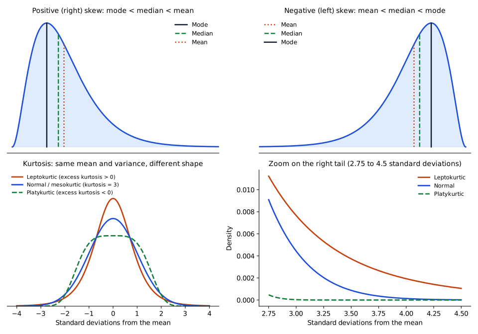
A symmetrical distribution looks the same on both sides of its mean; its mean, median and mode are equal. With symmetry, a loss interval (e.g., −6% to −4% around a zero mean) occurs as often as the matching gain interval (+4% to +6%). Skewness measures the lack of symmetry.
Key concept
| Shape | Long tail | Order of central measures | Sample skewness |
|---|---|---|---|
| Symmetrical | none | mean = median = mode | 0 |
| Positively skewed (skewed right) | right (large positive outliers) | mode < median < mean | > 0 |
| Negatively skewed (skewed left) | left (large negative outliers) | mean < median < mode | < 0 |
The mean is pulled toward the long tail because it is the measure most affected by outliers. In a skewed unimodal distribution, the median lies between the mode and the mean. For returns, positive skew means that more than half of the periods earn less than the mean (the median is below it), while a few periods bring very large gains. Negative skew is the mirror image: most periods earn more than the mean, and occasional large losses pull the mean down. Sample skewness averages the cubed standardized deviations, where is the sample standard deviation (the LOS asks for interpretation, not calculation):
Right-skewed data have positive sample skewness, since upside deviations from the mean are bigger on average. A quick way to judge the direction of skew is to compare the distance from the mode (peak) to each end of the range: the longer side is the tail.
Kurtosis
Kurtosis measures how peaked a distribution is and how thick its tails are, relative to a normal distribution (kurtosis ). Excess kurtosis kurtosis . Kurtosis uses the fourth power of the standardized deviations:
Key concept
| Term | Kurtosis | Excess kurtosis | Shape vs. normal |
|---|---|---|---|
| Leptokurtic | > 3 | > 0 (positive) | More peaked, fatter tails: more small deviations and more very large deviations from the mean |
| Mesokurtic | = 3 | = 0 | Same as normal |
| Platykurtic | < 3 | < 0 (negative) | Flatter (less peaked), thinner tails |
Fat tails matter for risk: a leptokurtic return distribution produces extreme outcomes (both large gains and large losses) more often than a normal model predicts. Actual asset returns tend to show both skewness and excess kurtosis, so risk models that assume normality understate the chance of extreme losses. In general, more negative skew and greater excess kurtosis both mean greater risk.
Common exam traps
- Dividing by when the data are a sample, or by when they are the whole population. For the four sample returns, dividing by 4 gives a standard deviation of 5.48% instead of 6.32%.
- Dividing the MAD by , or averaging the signed deviations, which always sum to zero. In the example, instead of 5.0%.
- Stopping at the variance when the standard deviation (its square root) is asked for. In the example, that answer is 40 (%²) instead of 6.32%.
- Comparing kurtosis with 0 instead of 3 (only excess kurtosis is compared with 0). A kurtosis of 2.5 is platykurtic even though the number is positive.
- Putting the mean on the wrong side: it is the largest of the three measures under positive skew and the smallest under negative skew.
- Reading one very low outlier (e.g. a single very poor score) as positive skew. It creates negative skew and pulls the mean below the median.
Exam shortcuts
- In a skewed unimodal distribution the median lies between the mode and the mean, and the mean lies on the side of the long tail, so the direction of skew fixes the order of all three measures.
Bottom line
- The range, maximum minus minimum, uses only the two extreme observations, while the mean absolute deviation averages the unsigned deviations from the mean.
- Sample variance divides the sum of squared deviations from the mean by (Bessel's correction), which makes an unbiased estimator of ; population variance divides by .
- Taking the positive square root of the variance gives the standard deviation, which is in the same units as the data, while the variance is in squared units.
- Under the root of time law, with independent returns the variance over periods is and the standard deviation is , although long-horizon variance is often lower in practice.
- A positively skewed distribution has a long right tail with mode < median < mean, a negatively skewed one has a long left tail with mean < median < mode, and a symmetrical one has all three equal.
- A normal distribution has kurtosis 3; excess kurtosis is kurtosis − 3, a leptokurtic distribution (above 3) has fatter tails, and more negative skew and greater excess kurtosis both mean greater risk.
Quick check
A histogram of a biotech fund's daily returns shows a long tail stretching to the right, created by a few very large gains. For this unimodal distribution, which relationship among the measures of central tendency is most likely?
Show answer and explanation
Correct answer: C
A long right tail means the distribution is positively skewed. The large positive outliers pull the mean upward the most, the median less, and the mode (the peak) not at all, so mean > median > mode.
Why the other options are wrong
- A. This ordering describes a negatively skewed distribution with a long left tail.
- B. Equality of the three measures describes a symmetrical distribution, which has no long tail.
Key takeaway Positive (right) skew: mode < median < mean.
Module 5.3
Covariance, Correlation, and Alternative Measures of Dispersion
LOS 5.c — Covariance and correlation
Scatter plots
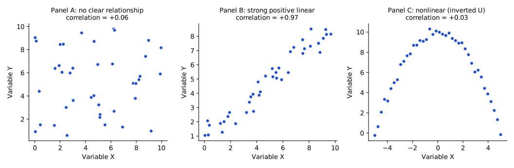
A scatter plot graphs paired observations of two variables, one on each axis. It shows at a glance whether the variables move together, whether the relationship is roughly a straight line, and whether there is a nonlinear relationship that a correlation coefficient would miss.
Covariance
Covariance measures how two variables move together:
(The population version uses the population means and divides by .) A positive covariance means the variables tend to be above (or below) their means at the same time; a negative covariance means they tend to move in opposite directions.
Example. Four annual returns on fund X are 6%, −2%, 10% and 2%, and on fund Y 5%, 1%, 9% and 1%. Both means are 4%.
- Deviations from the means (percentage points): fund X gives 2, −6, 6, −2; fund Y gives 1, −3, 5, −3.
- Multiply each pair and add: .
- Divide by : (%²).
Every cross-product is positive, so the two funds were above or below their means in the same years.
Covariance is hard to interpret: its size depends on the units of the data, and its units are the product of the two variables' units (e.g. percent squared). A covariance of 30 shows only the direction of co-movement; it says nothing about how strong it is. Covariance has no upper or lower bound. The covariance of a variable with itself is its variance: .
Correlation
The correlation coefficient (correlation) standardizes covariance by the two standard deviations:
Key concept
Here and are the sample standard deviations. The population version uses and in the same way.
Key concept
| Value | Interpretation |
|---|---|
| Perfect positive correlation: deviations from the mean move in exact proportion, same direction; all points lie on one upward-sloping straight line, however steep or flat | |
| Positive linear association; strength grows as approaches 1 | |
| No linear relationship | |
| Negative linear association | |
| Perfect negative correlation: all points lie on one downward-sloping straight line |
Correlation has no units and always lies between −1 and +1. It is not a probability: does not mean "a 60% chance the variables move in opposite directions." Because the covariance is divided by the two standard deviations, the correlation moves further from zero when the standard deviations shrink and the covariance stays the same.
Example. Returns on two funds have variances of 0.0036 and 0.0100 and a covariance of 0.0021. Standard deviations are and , so
This is a positive but modest linear association. The variances must be converted to standard deviations first.
For the four years of fund returns in the covariance example, and , so , a strong positive linear association.
Limits of correlation
- Correlation is not causation. A strong correlation does not show that one variable drives the other, or which way any causality runs. Say the variables show a positive (or negative) association and investigate cause separately.
- Outliers can create or destroy a correlation; check whether removing them changes the result materially and whether they are information or noise.
- Spurious correlation is correlation that arises by chance, or because both variables are related to a third variable (e.g., two series that both trend upward with inflation or population), with no causal link between them.
LOS 5.d — Downside risk and relative dispersion
Semivariance and target downside deviation
Variance and standard deviation treat deviations above and below the mean alike. In some situations it is more useful to count only outcomes below the mean or below a chosen target, which measures downside risk.
- Semivariance: a variance built only from the outcomes that fall below the mean. The squared deviations of the below-mean observations are summed and divided by the sample size:
Its square root is the semideviation, a downside counterpart of the standard deviation.
- Target downside deviation (also target semideviation): like a standard deviation, but only outcomes below a chosen target contribute; the denominator is still the full sample size minus one:
Example. Five annual returns: 12%, −4%, 7%, 3%, 10%; target 6%. Only −4% and 3% are below target: squared shortfalls . . Raising the target to 8% brings the 7% return into the count and makes the other two shortfalls larger: . A higher target never lowers the target downside deviation.
Coefficient of variation
Comparing standard deviations of assets with very different mean returns can mislead. A relative dispersion measure scales risk by the mean. The coefficient of variation (CV) is:
Key concept
It measures risk per unit of mean return, so a lower CV is better (less risk per unit of return). Because it is a ratio of two numbers in the same units, it is unit-free and can be quoted as a decimal or a percentage. The Sharpe ratio (Reading 8) turns the CV around: it divides the excess return over the risk-free rate by the standard deviation. With a zero risk-free rate, the CV is simply the inverse of the Sharpe ratio. When a Sharpe ratio and a risk-free rate are given, first recover , then divide by the mean.
Example. Fund M has a mean of 5% and a standard deviation of 4%, so . Fund N has a mean of 11% and a standard deviation of 7.7%, so . Fund N has the higher standard deviation but the better (lower) CV.
| Measure | Uses | Scale |
|---|---|---|
| Standard deviation | All deviations from the mean | Absolute (units of the data) |
| Target downside deviation | Only shortfalls below a target | Absolute |
| Coefficient of variation | Standard deviation ÷ mean | Relative (per unit of return) |
Common exam traps
- Inverting the CV or using the variance. CV standard deviation ÷ mean; when a variance is given, take its square root first. For fund M, inverting gives and using the variance of 16 (%²) gives 3.20, instead of 0.80.
- Subtracting a risk-free rate given in the question. The CV uses the mean itself; excess return over standard deviation is a Sharpe-type ratio, a different measure.
- Picking the asset with the lowest standard deviation as the best risk-return tradeoff, or the one with the highest standard deviation as the highest relative risk. Both are judged by the CV.
- Dividing the covariance by one variance (a slope-type ratio) or by the product of the variances, instead of by the product of the standard deviations. In the two-fund example, and , instead of 0.35.
- Reading a correlation near zero as proof that the variables are unrelated. It rules out only a linear relationship.
- Dividing the target downside deviation by the number of below-target outcomes (or that number minus one) instead of the full sample size minus one. In the 6% target example, instead of .
Exam shortcuts
- With a zero risk-free rate the CV is the inverse of the Sharpe ratio, so one can be read straight from the other.
- A higher target never lowers the target downside deviation, which rules out an answer in which raising the target reduces it.
Bottom line
- Sample covariance is ; its sign shows the direction of co-movement, but its size depends on the units and it has no upper or lower bound.
- Correlation has no units, lies between −1 and +1, and means no linear relationship.
- Correlation is not causation, outliers can create or destroy a correlation, and spurious correlation arises by chance or because both variables are related to a third variable.
- A scatter plot can reveal a nonlinear relationship that a correlation coefficient would miss.
- Semivariance uses only the outcomes below the mean, and the target downside deviation uses only the outcomes below a target but keeps the full sample size minus one in the denominator.
- The coefficient of variation measures risk per unit of mean return, is unit-free, and a lower CV is better.
Quick check
The covariance between the returns on Norland Utilities and Quarry Point Materials is 21.6 (percent squared). The standard deviation of Norland's returns is 8% and that of Quarry Point's returns is 6%. The correlation coefficient of the two return series is closest to:
Show answer and explanation
Correct answer: B
Correlation standardizes covariance by dividing it by the product of the two standard deviations.
Why the other options are wrong
- A. +0.34 divides the covariance by Norland's variance only ().
- C. +0.60 divides the covariance by Quarry Point's variance only ().
Key takeaway ; dividing by a single variance gives a slope-type ratio.
Practice Questions
Priya Raman plans to model the monthly percentage changes in a copper price index. Her statistical tests will be most reliable if the series is stationary, which means that:
Show answer and explanation
Correct answer: C
Data are stationary when the mean and variance of the underlying distribution stay constant through time. When these characteristics shift, the series is nonstationary, and inferences about future outcomes drawn from past data become unreliable. For this reason analysts usually model percentage changes rather than trending price levels.
Why the other options are wrong
- A. The geometric and arithmetic means coincide only when every observation is identical; that has nothing to do with stationarity.
- B. The median always lies inside the interquartile range, and the mean usually does unless the data are extremely skewed. This says nothing about whether the distribution is stable over time.
Key takeaway Stationary = stable mean and variance over time. Price levels are usually nonstationary; returns (percentage changes) are more likely to be stationary.
A multi-asset portfolio produced the returns shown below over the last four years.
| Year | Return |
|---|---|
| 1 | 19.0% |
| 2 | 7.5% |
| 3 | −9.6% |
| 4 | 4.9% |
Treating these returns as a sample, their coefficient of variation is closest to:
Show answer and explanation
Correct answer: C
The coefficient of variation is the sample standard deviation divided by the mean return. Because the returns are a sample, the standard deviation uses in the denominator.
Mean .
| Year | Return | (Return − 5.45) |
|---|---|---|
| 1 | 19.0 | 183.60 |
| 2 | 7.5 | 4.20 |
| 3 | −9.6 | 226.50 |
| 4 | 4.9 | 0.30 |
| Sum | 414.61 |
Why the other options are wrong
- A. 0.46 inverts the ratio: .
- B. 1.87 uses the population standard deviation, , giving ; the returns are to be treated as a sample.
Key takeaway Sample coefficient of variation: compute s with n − 1, then divide by the mean.
This reading has 60 questions in the full bank. Practice all of them.
Key Takeaways
- Compute all three measures explicitly; the mean is rarely exactly equal to an observed value.
- Stationary = stable mean and variance over time. Price levels are usually nonstationary; returns (percentage changes) are more likely to be stationary.
- Positive (right) skew: mode < median < mean.
- ; dividing by a single variance gives a slope-type ratio.
- Sample coefficient of variation: compute s with n − 1, then divide by the mean.