Quantitative Methods · Reading 4

Time Value of Money

CFA Level I · Quantitative Methods · Reading 4: The Time Value of Money in Finance · about 49 min

Quantitative Methods notes as a PDF166 pages · 2.6 MB · free, no sign-up · All PDFs

What you'll learn

LOS 4.a Calculate and interpret the present value of fixed-income instruments (zero-coupon, coupon, perpetual, amortizing) and equity instruments (preferred stock, constant-growth and multistage DDM) from their expected cash flows.
LOS 4.b Calculate and interpret the implied return of fixed-income instruments and the implied required return and growth rate of equity, given price and cash flows.
LOS 4.c Explain the cash flow additivity principle and the no-arbitrage condition, and use them to derive implied forward interest rates, forward exchange rates and option values.

Module 4.1

Discounted Cash Flow Valuation

This reading prices fixed-income and equity instruments as the present value of their expected cash flows and then works the same relationships backward to find implied returns and growth rates. It closes with cash flow additivity and the no-arbitrage principle, which give forward interest rates, forward exchange rates and the value of an option in a one-period binomial model. Most of the calculations use the financial calculator's TVM worksheet.

LOS 4.a — Present value of fixed-income and equity instruments

1. The time value of money

The time value of money means a given amount of money today is worth more than the same amount in the future. To give up money now, investors must expect a rate of return; that same rate, used as a discount rate, converts future cash flows into a present value (PV) and present amounts into a future value (FV).

Key concept

F V = P V (1 + r)^{t} P V = \frac{F V}{( 1 + r ) ^{t}}

where $r$ is the rate per compounding period and $t$ is the number of periods. With continuous compounding: $F V = P V e^{r t}$ and $P V = F V e^{- r t}$ .

Financial calculator (TI BA II Plus, P/Y = C/Y = 1 and END mode unless stated) keys: N = number of periods, I/Y = rate per period (in %), PV = present value, PMT = constant periodic payment, FV = future value, CPT = compute. Enter outflows as negative and inflows as positive (e.g., price paid negative, face value received positive). Clear the TVM worksheet between problems.

With $m$ compounding periods a year, use the rate $r / m$ and years $\times m$ periods. Unequal cash flows are moved to the target date one at a time and added: at 6% compounded semiannually, 2,000 paid at the end of year 1 is worth $2, 000 \times 1.0 3^{4} = 2, 251.02$ at the end of year 3.

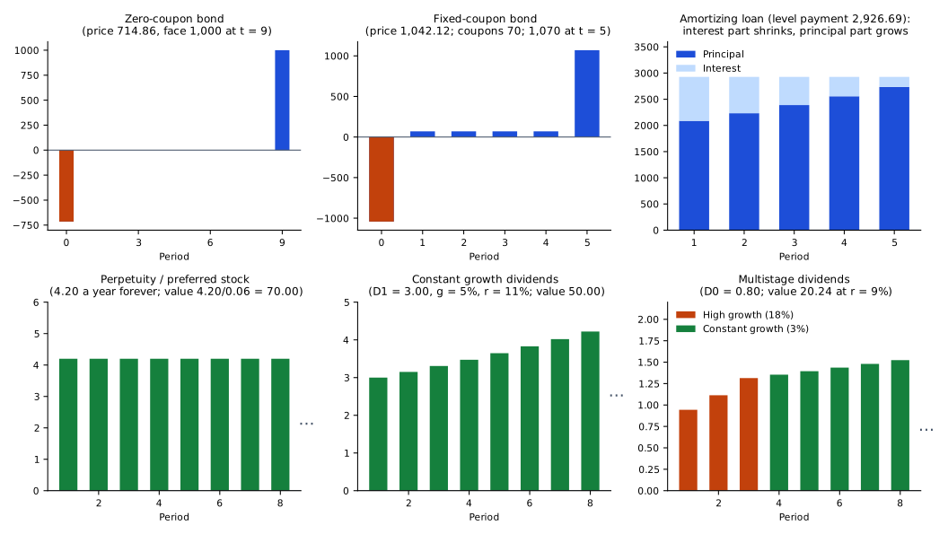
The instruments below differ only in the pattern of their cash flows:

Six panels. Zero-coupon bond: pay 714.86 at t = 0, receive 1,000 at t = 9. Fixed-coupon bond: pay 1,042.12 at t = 0, receive 70 at t = 1 to 4 and 1,070 at t = 5. Amortizing loan: five level payments of 2,926.69, with the interest part falling from 840.00 to 191.47 and the principal part rising from 2,086.69 to 2,735.22. Perpetuity or preferred stock: 4.20 every year forever, value 70.00 at 6%. Constant growth dividends: 3.00 growing 5% a year, value 50.00 at 11%. Multistage dividends: from 0.80, growing 18% for three years (0.94, 1.11, 1.31) then 3% a year, value 20.24 at 9%. — Cash flow patterns of the instruments in this module (numbers from the module's examples)

2. Fixed-income instruments

Pure discount instruments

A pure discount instrument (zero-coupon bond) is bought for less than its face value, and the investor receives the face value at maturity; the difference is the interest earned. Its price is set by two inputs: the time left to maturity and the yield to maturity, which is the rate used to discount the face value.

Example. A $1,000 face value bond with 9 years to maturity and a yield of 3.8% is priced at $1, 000/1.03 8^{9} = $714.86$ (N = 9, I/Y = 3.8, PMT = 0, FV = 1,000, CPT PV = −714.86).

If the yield is negative, the zero-coupon bond is priced at a premium (above face value): at −0.4% the same bond costs $1, 000/0.99 6^{9} = $1, 036.73$ .

Fixed-coupon bonds

For a fixed-coupon bond, the coupon rate × face value sets the coupon (PMT). The yield to maturity (I/Y) is the rate that, used to discount the bond's cash flows, reproduces its price. The two rates generally differ. The price is the PV of the coupons and the face value, all discounted at the YTM:

P = t = 1 \sum N \frac{C}{( 1 + Y T M ) ^{t}} + \frac{F}{( 1 + Y T M ) ^{N}}

Example. A 5-year, $1,000 bond with a 7% annual coupon and a YTM of 6%: N = 5, I/Y = 6, PMT = 70, FV = 1,000, CPT PV = −1,042.12.

Key concept

Relationship	Price vs. par
Coupon rate > YTM	Premium (price > par)
Coupon rate = YTM	Par
Coupon rate < YTM	Discount (price < par)

A floating-rate bond resets its coupon to a market reference rate plus a fixed margin (e.g., reference 2.5% + 150 basis points = 4.0%); one basis point = 0.01%.

Perpetual bonds

A perpetual bond (a perpetuity) pays a fixed amount forever and has no maturity:

P V_{perpetuity} = \frac{P M T}{r}

The first payment is assumed to arrive one period from now.

Amortizing bonds and annuities

An annuity is a series of equal payments at equal intervals. The formulas below assume that each payment comes at the end of its period, so the first payment is one period away. An amortizing bond (or a fixed-rate mortgage) pays a constant amount that includes both interest and principal. As the outstanding balance falls, the interest portion of each payment declines and the principal portion increases. Whether the early payments are mostly interest depends on the rate and the term (with a low rate or a short term, even the first payment can be mostly principal).

P V_{annuity} = P M T \times \frac{1 - ( 1 + r ) ^{- N}}{r} P M T = \frac{r \times P V}{1 - ( 1 + r ) ^{- N}}

Example. A $12,000 loan at 7% repaid with 5 equal year-end payments: N = 5, I/Y = 7, PV = 12,000, FV = 0, CPT PMT = −2,926.69. For monthly payments use N = years × 12 and I/Y = annual rate ÷ 12.

To split a payment into interest and principal:

Interest $= r \times$ the balance at the start of the period.
Principal repaid $=$ payment $-$ interest.
New balance $=$ old balance $-$ principal repaid.

For this loan, the first payment carries interest of $0.07 \times 12, 000 = $840.00$ and repays $2, 926.69 - 840.00 = $2, 086.69$ of principal, leaving $9,913.31. The second carries interest of $0.07 \times 9, 913.31 = $693.93$ and repays $2,232.76. The interest part falls each year by exactly the amount the principal part rises. The full schedule for the loan:

Amortization schedule: $12,000 at 7%, five year-end payments

Year	Beginning balance	Payment	Interest (7%)	Principal repaid	Ending balance
1	12,000.00	2,926.69	840.00	2,086.69	9,913.31
2	9,913.31	2,926.69	693.93	2,232.76	7,680.56
3	7,680.56	2,926.69	537.64	2,389.05	5,291.51
4	5,291.51	2,926.69	370.41	2,556.28	2,735.22
5	2,735.22	2,926.69	191.47	2,735.22	0.00

Annuities that start later

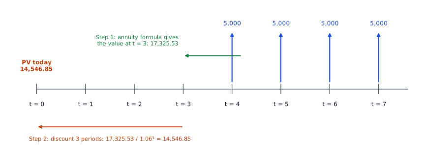
The annuity formula gives a value one period before the first payment. For a later first payment:

Apply the annuity formula (value one period before the first payment).
Discount that value to today as a single sum.

Example. Four payments of 5,000 start at $t = 4$ , and the rate is 6%. Step 1 gives $5, 000 \times [1 - 1.0 6^{- 4}] /0.06 = 17, 325.53$ at $t = 3$ . Step 2 gives $17, 325.53/1.0 6^{3} = 14, 546.85$ today.

Timeline t = 0 to t = 7 with payments of 5,000 at t = 4, 5, 6 and 7. Step 1: the annuity formula gives 17,325.53 at t = 3. Step 2: discounting three periods at 6% gives 14,546.85 today. — Valuing an annuity whose first payment is at t = 4

3. Equity instruments

Equity securities are valued as the PV of expected future cash flows discounted at the investor's required return, the return that induces investors to hold the share. Equity usually has no maturity, and its cash flows can vary.

Preferred stock pays a fixed dividend (a stated percentage of par value) indefinitely, so it is valued as a perpetuity:

V_{preferred} = \frac{D _{p}}{r _{p}}

where $D_{p}$ is the dividend per period and $r_{p}$ is the market's required return on the preferred stock.

Example. A $4.20 annual dividend and a 6% required return give a value of $70.00. The stated dividend rate sets the cash flow; the required return is the discount rate.

Common stock is a residual claim on the company's assets after all other claims are met. Dividends are not promised; management decides whether and when to pay them. The dividend discount models (DDMs):

Constant dividend: value the share as a perpetuity, as with preferred stock.
Constant growth DDM (Gordon growth model):

V_{0} = \frac{D _{1}}{r _{e} - g _{c}}, D_{1} = D_{0} (1 + g_{c})

Here $V_{0}$ is the value of all dividends from $D_{1}$ onward, $r_{e}$ is the required return on common equity and $g_{c}$ is the constant growth rate of dividends. The model needs the dividend expected next period ( $D_{1}$ ), a constant growth rate, and $r_{e} > g_{c}$ . Example. With $D_{1} = $3.00$ , $r_{e} = 11%$ and $g_{c} = 5%$ , $V_{0} = 3.00/0.06 = $50.00$ .

Multistage DDM: forecast the dividends of a high-growth phase individually, then apply the Gordon model at the start of the constant-growth phase. The Gordon model gives a value one period before the dividend in its numerator: $P_{n} = D_{n + 1} / (r_{e} - g_{c})$ . The high-growth rate may be above $r_{e}$ , because those dividends are discounted one at a time (18% against 9% in the example below). Only the constant growth rate used in the Gordon step must be below $r_{e}$ .

Multistage example. $D_{0} = $0.80$ , growth 18% for 3 years, then 3% forever, $r_{e} = 9%$ .
$D_{1} = 0.944, D_{2} = 1.1139, D_{3} = 1.3144, D_{4} = 1.3144 \times 1.03 = 1.3539$
$P_{3} = 1.3539/ (0.09 - 0.03) = 22.564$

V_{0} = \frac{0.944}{1.09} + \frac{1.1139}{1.0 9 ^{2}} + \frac{1.3144 + 22.564}{1.0 9 ^{3}} = $20.24

Worked example: pricing a bond and splitting a loan payment

A 5-year bond has a $1,000 face value, a 5.25% annual coupon and a YTM of 4.35%. Separately, a borrower takes a $250,000 loan at 4.8%, repaid with 10 equal year-end payments.

Step 1. The coupon rate (5.25%) is above the YTM (4.35%), so the bond must sell at a premium.

Step 2. Price the bond: N = 5; I/Y = 4.35; PMT = 52.50; FV = 1,000; CPT PV = −1,039.68. The price is $1,039.68, above par as predicted.

Step 3. One year later, with the YTM unchanged: N = 4; I/Y = 4.35; PMT = 52.50; FV = 1,000; CPT PV = −1,032.40. The price is still above par, but closer to it.

Step 4. Loan payment: N = 10; I/Y = 4.8; PV = 250,000; FV = 0; CPT PMT = −32,062.44.

Step 5. First payment: interest $0.048 \times 250, 000 = $12, 000.00$ ; principal $32, 062.44 - 12, 000.00 = $20, 062.44$ ; new balance $229,937.56.

Step 6. Second payment: interest $0.048 \times 229, 937.56 = $11, 037.00$ ; principal $32, 062.44 - 11, 037.00 = $21, 025.44$ . The interest part fell by $963.00 and the principal part rose by the same amount.

Result. The bond is priced at $1,039.68. The loan payment is $32,062.44, of which $12,000.00 is interest in year 1 and $11,037.00 in year 2.

Common exam traps

Mixing up the coupon rate (which sets PMT) and the YTM (which is I/Y), or, when the bond's own price is given, taking the yield on similar bonds as its YTM.
Annuities and single sums: confusing a present value with a future value, adding up payments without discounting them, or discounting with simple interest, $F V / (1 + r t)$ , which ignores compounding.
Perpetuity value = payment ÷ rate, which is already today's value when the first payment is one period away. Multiplying instead, or discounting that value one more period, gives a wrong value. With the $4.20 dividend and 6% required return above, discounting the $70.00 value one more period gives $66.04.
Gordon model: using $D_{0}$ where $D_{1}$ is needed, or applying the model when growth is not constant or not below the required return.
Multistage DDM: the terminal value $P_{n}$ uses $D_{n + 1}$ and is discounted $n$ periods, not $n + 1$ . In the multistage example, discounting $P_{3}$ four periods gives $18.80 instead of $20.24.
Annuity that starts later: discounting over the full number of periods to the first payment instead of one period fewer. In the example, discounting 17,325.53 four periods gives 13,723.44 instead of 14,546.85.
Forgetting that a negative yield gives a price above face value.
Monthly loans: converting only one of N and I/Y to months.

Exam shortcuts

Compare the coupon rate with the YTM before calculating a bond price: a coupon above the YTM means a premium, equal means par, below means a discount, so prices on the wrong side of par can be ruled out at once.
A zero-coupon bond, a coupon bond and a level loan are all one TVM entry; a zero is the same entry with PMT = 0.
A level perpetuity or a preferred share needs no worksheet: value = payment ÷ rate.

Bottom line

Every instrument here is valued as the present value of its expected cash flows, each discounted with $P V = F V / (1 + r)^{t}$ .
A bond sells at a premium when its coupon rate is above its YTM, at par when they are equal and at a discount when the coupon rate is below the YTM.
A perpetuity is worth $P M T / r$ one period before its first payment, and preferred stock is valued the same way, $D_{p} / r_{p}$ .
In an amortizing loan each payment's interest is the rate times the opening balance, so the interest part falls and the principal part rises over the life of the loan.
The Gordon growth model $V_{0} = D_{1} / (r_{e} - g_{c})$ uses next period's dividend and requires constant growth below the required return.
In a multistage DDM the terminal value $P_{n} = D_{n + 1} / (r_{e} - g_{c})$ is discounted $n$ periods, together with the dividend paid at $n$ .

Quick check

Question 1Core

Brisa Therapeutics expects to receive the licensing fees shown in the table below. Its finance team discounts them at a stated annual rate of 6%, compounded monthly. The present value of the three fees today is closest to:

Expected licensing fees

Received at the end of year	Fee
1	$5,000
2	$9,000
3	$12,000

Show answer and explanation

Correct answer: A

The fees are unequal, so each one is discounted to today on its own and the present values are added. With monthly compounding, the rate per period is 6%/12 = 0.5% and each year has 12 periods, so the fees are discounted over 12, 24 and 36 months.

P V = \frac{5 , 000}{1.00 5 ^{12}} + \frac{9 , 000}{1.00 5 ^{24}} + \frac{12 , 000}{1.00 5 ^{36}}

= 4, 709.53 + 7, 984.67 + 10, 027.74 = $22, 721.94

Calculator (P/Y = C/Y = 1, END mode), first fee: N = 12; I/Y = 0.5; PMT = 0; FV = 5,000; CPT PV = −4,709.53. Then N = 24; FV = 9,000; CPT PV = −7,984.67, and N = 36; FV = 12,000; CPT PV = −10,027.74.

Why the other options are wrong

B. $22,802 discounts at 6% with annual compounding ( $1.06$ , $1.0 6^{2}$ and $1.0 6^{3}$ ). Monthly compounding raises the effective annual rate to $1.00 5^{12} - 1 = 6.17%$ , so the present value is lower.
C. $25,708 uses the monthly rate of 0.5% but discounts over only 1, 2 and 3 periods, counting years instead of months.

Key takeaway With $m$ compounding periods a year, discount at $r / m$ over $m \times$ years periods, and value unequal cash flows one at a time.

Module 4.2

Implied Returns and Cash Flow Additivity

LOS 4.b — Implied returns and implied growth

The PV relationships from Module 4.1 can be rearranged to solve for the rate of return implied by a known price and known (or assumed) cash flows.

Zero-coupon bond

r = (\frac{F V}{P V})^{1/ N} - 1

Example. A $1,000 face value bond maturing in 6 years and priced at $820 yields $(1, 000/820)^{1/6} - 1 = 3.36%$ (N = 6, PV = −820, PMT = 0, FV = 1,000, CPT I/Y = 3.36).

Coupon bond

The yield to maturity of a coupon bond generally has no closed-form solution, so it is found with the calculator: N, PMT = coupon, FV = face, PV = −price, CPT I/Y. Example. A 5-year, $1,000 par bond with a 4% annual coupon priced at $975.00: N = 5, PMT = 40, FV = 1,000, PV = −975, CPT I/Y = 4.57.

Price and yield move in opposite directions: when a bond's price rises, its YTM falls, and when the price falls, its YTM rises. If the bond above rises to $990.00, its YTM falls to 4.23%.

Equity: implied required return

The required return on equity cannot be observed directly. Rearranging the constant growth DDM with the observed price gives:

Key concept

r_{e} = \frac{D _{1}}{P _{0}} + g_{c} = dividend yield + constant growth rate

The dividend yield here is the expected dividend divided by the current price.

Equity: implied growth rate

Given a required return, the implied growth rate is

g_{c} = r_{e} - \frac{D _{1}}{P _{0}} = required return - dividend yield

When the required return is the unknown and the dividend given is the one just paid ( $D_{0}$ ), first convert it: $D_{1} = D_{0} (1 + g_{c})$ .

Given	Solve for	Formula
$P_{0}, D_{1}, g_{c}$	Required return	$D_{1} / P_{0} + g_{c}$
$P_{0}, D_{1}, r_{e}$	Implied growth	$r_{e} - D_{1} / P_{0}$
$r_{e}, g_{c}, P_{0}$	Dividend yield	$r_{e} - g_{c}$

Example. A share priced at $50.00 is expected to pay a $2.00 dividend next year, a dividend yield of 4.0%. With 5% constant growth, the implied required return is 4.0% + 5% = 9.0%. If investors instead require 10%, the implied growth rate is 10% − 4.0% = 6.0%.

LOS 4.c — Cash flow additivity, no arbitrage and their uses

1. Cash flow additivity principle

Under the cash flow additivity principle, the value of a stream of cash flows equals the total obtained by discounting each cash flow separately and adding the results. Streams can be added together (combining cash flows that fall on the same date) or split into pieces in any way, and the PVs of the pieces add up to the PV of the whole.

Example. At 8%, payments of $200, $200, $500 and $200 at the ends of years 1–4 are worth the same as a 4-year annuity of $200 (PV = 662.43) plus a single $300 at year 3 (PV = 238.15), a total of $900.58. This is replication: an annuity plus a zero-coupon bond recreates the uneven stream. Splitting off an annuity equal to the smallest (or any) level amount leaves a residual stream in the same time order. The order matters, because earlier cash flows are worth more.

To compare two projects, subtract one stream from the other date by date. If the difference is $+ X$ earlier and $- X$ later, the project with the earlier cash flow has the higher PV at any positive discount rate, with no NPV calculation needed.

2. No-arbitrage principle (law of one price)

Additivity underpins the no-arbitrage principle (the law of one price): two assets whose future cash flows match in every possible state must sell for the same price now. When their prices diverge, traders buy the cheaper asset and sell the dearer one, and that trading pushes the two prices back together. Such gaps close fast, so an arbitrageur must act at once.

The principle is applied below to derive forward interest rates and forward exchange rates and to value options.

3. Forward interest rates

A spot rate $S_{n}$ is the annualized rate for a loan made today for $n$ years. A forward rate is for a loan made at a future date: 1y1y is a 1-year rate one year from now, 2y1y a 1-year rate two years from now, 3y2y a 2-year rate three years from now. Borrowing or investing over the same horizon by any route must cost the same:

Key concept

(1 + S_{2})^{2} = (1 + S_{1}) (1 + 1 y 1 y) \Rightarrow 1 y 1 y = \frac{( 1 + S _{2} ) ^{2}}{1 + S _{1}} - 1

(1 + S_{3})^{3} = (1 + S_{1}) (1 + 1 y 1 y) (1 + 2 y 1 y)

A forward rate solved from spot rates in this way is an implied forward rate. Example. With $S_{1} = 1.5%$ and $S_{2} = 2.5%$ , $1 y 1 y = 1.02 5^{2} /1.015 - 1 = 3.51%$ . With an upward-sloping spot curve, the forward rate lies above both spot rates. An investor is indifferent between the 2-year bond and rolling 1-year bonds at $S_{1}$ then 1y1y.

Two ways to invest for two years: a 2-year spot bond, or a 1-year spot bond followed by the 1y1y forward rate

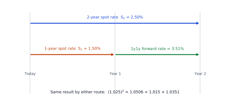
If an investor could instead lock in 4.00% for the second year, the two routes would no longer cost the same. Borrowing $1,000,000 for two years at $S_{2}$ means repaying $1, 000, 000 \times 1.02 5^{2} = $1, 050, 625$ . Lending the same amount for one year at 1.5% and then for one more year at the locked-in 4.00% returns $1, 000, 000 \times 1.015 \times 1.04 = $1, 055, 600$ . The $4,975 gain at year 2 needs none of the investor's own money and carries no risk, so it is an arbitrage profit. Traders exploiting it push the forward rate back to 3.51%.

Longer forward rates follow the same rule. For the 2-year rate one year from now, $(1 + S_{3})^{3} = (1 + S_{1}) (1 + 1 y 2 y)^{2}$ .

4. Forward exchange rates

An exchange rate states how many units of one currency are needed to buy one unit of another. A rate quoted as A/B is the price of one unit of B (the base currency) in units of A (the price currency). No arbitrage links forward and spot rates to the two riskless interest rates for the forward's horizon. If the forward rate were out of line, a trader could borrow one currency, convert it at the spot rate, invest it at the other currency's riskless rate and sell the proceeds forward, locking in a riskless profit. Use one of two equivalent forms, depending on how the rates are quoted:

With annual rates and a horizon of $T$ years:

\frac{Forward}{Spot} = \frac{( 1 + r _{price} ) ^{T}}{( 1 + r _{base} ) ^{T}}

With rates already stated for the forward's period (e.g., a 90-day money-market rate converted as $r \times 90/360$ ), no exponent is applied:

\frac{Forward}{Spot} = \frac{1 + r _{price, period}}{1 + r _{base, period}}

The percentage difference between forward and spot is approximately the interest rate differential. Example. For a one-year forward with spot at 1.1000 USD/EUR, a one-year USD rate of 4% and a one-year EUR rate of 2%, the forward rate is $1.1000 \times 1.04/1.02 = 1.1216$ , about 1.96% above spot, close to the 2% differential. The currency with the higher interest rate trades at a forward discount.

5. Option values: one-period binomial model

An option gives its holder the right to buy (call option) or sell (put option) an asset at a set exercise price, with no obligation to do so. At expiration: call value $= max (S_{T} - X, 0)$ ; put value $= max (X - S_{T}, 0)$ . At expiration, an option is out of the money when exercising would not pay (a call whose exercise price is above the market price, or a put whose exercise price is below it), so the holder lets it expire. An option that is in the money at expiration is exercised.

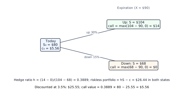
In a binomial model, the underlying moves to one of two prices over the period. A one-period model needs the underlying's value today, the exercise price (the option expires at the end of the period), the returns in an up move and a down move, and the risk-free rate for the period. Write one call and buy $h$ shares so that the portfolio's value is the same after an up or down move (risk free):

h = \frac{c _{u} - c _{d}}{S _{u} - S _{d}}

This $h$ is the hedge ratio: the number of shares bought per option written.

The riskless portfolio must earn the risk-free rate, so: value today $= \frac{h S _{d} - c _{d}}{1 + R _{f}}$ , and the option value is $c_{0} = h S_{0} - portfolio value today$ .

Example. $S_{0} = $80$ , up 30% to $104, down 15% to $68, $X = $90$ , $R_{f} = 3.5%$ . Call payoffs: $14 (up) and $0 (down). $h = 14/36 = 0.3889$ . Portfolio at expiration $= 0.3889 \times 68 = $26.44$ in both states. PV $= 26.44/1.035 = $25.55$ . Call value $= 0.3889 \times 80 - 25.55 = $5.56$ .

One-period binomial tree for the call example: prices, payoffs, hedge ratio and call value

Common exam traps

Setting a price limit the wrong way round: for a zero, a return above X% requires a price below the one that gives X%.
Adding the dividend yield to the required return to get implied growth; the dividend yield is subtracted. With a 10% required return and a 4.0% dividend yield, that error gives 14.0% instead of 6.0%.
Averaging spot rates to get a forward rate. The forward rate comes from the compounded (geometric) relationship. With $S_{1} = 1.5%$ and $S_{2} = 2.5%$ , the average is 2.0%, while 1y1y is 3.51%.
Forward FX: taking the sum or the average of the two interest rates as the forward premium or discount, or putting the base-currency rate in the numerator of the exact ratio. With spot at 1.1000 USD/EUR, putting the EUR rate on top gives $1.1000 \times 1.02/1.04 = 1.0788$ instead of 1.1216.
Additivity: writing the residual cash flows in reverse date order, which changes their PV.
Binomial model: weighting the payoffs 50/50, discounting the hedged portfolio at a rate other than the risk-free rate, or reporting the portfolio's PV as the option value instead of subtracting it from the share position. In the example, weighting the payoffs 50/50 gives $0.5 \times 14/1.035 = $6.76$ and reporting the portfolio's PV gives $25.55, while the call is worth $5.56.

Exam shortcuts

With an upward-sloping spot curve the implied forward rate lies above both spot rates, so a forward rate between the two spot rates can be ruled out.
Check the direction of a forward exchange rate first: when the price currency has the higher interest rate the forward is above spot, and when it has the lower rate the forward is below spot.
When two cash flow streams differ only by $+ X$ earlier and $- X$ later, the stream with the earlier cash flow has the higher PV at any positive discount rate, with no NPV calculation needed.

Bottom line

The implied return on a zero-coupon bond is $(F V / P V)^{1/ N} - 1$ ; a coupon bond's YTM is found with the calculator (CPT I/Y).
A bond's price and its YTM move in opposite directions.
Rearranging the Gordon model gives the required return $r_{e} = D_{1} / P_{0} + g_{c}$ and the implied growth rate $g_{c} = r_{e} - D_{1} / P_{0}$ .
Under cash flow additivity the PV of a stream equals the sum of the PVs of its pieces, so an uneven stream can be replicated with annuities and zero-coupon bonds.
No arbitrage sets the implied forward rate $1 y 1 y = (1 + S_{2})^{2} / (1 + S_{1}) - 1$ and the forward exchange rate $Forward / Spot = (1 + r_{price})^{T} / (1 + r_{base})^{T}$ .
In a one-period binomial model the hedge ratio is $h = (c_{u} - c_{d}) / (S_{u} - S_{d})$ , the hedged portfolio earns the risk-free rate, and $c_{0} = h S_{0}$ minus the PV of the hedged portfolio.

Quick check

Question 2Core

Chiara Lombardi holds a 7-year corporate bond with a 5.3% annual coupon. Her monthly statement shows that the bond's yield to maturity rose from 5.1% last month to 5.6% this month. Over the month, the bond's price has most likely:

Show answer and explanation

Correct answer: A

Price and yield to maturity are inversely related. The yield to maturity is the discount rate that equates the bond's cash flows with its price. A higher yield means the same fixed cash flows are discounted more heavily, so the price must have fallen.

Why the other options are wrong

B. A price increase would go with a lower yield to maturity, not a higher one.
C. A flat price would leave the yield to maturity almost unchanged (only the passage of one month would move it slightly). It could not produce a 0.5 percentage point rise.

Key takeaway Price and YTM are inversely related: when the yield rises, the price falls.

Practice Questions

Question 3Core

Brightwater Utilities has preferred stock outstanding that pays a fixed annual dividend of $2.60 per share with no maturity date. An investor who requires a 7.2% rate of return should be willing to pay, per share, a maximum of closest to:

Show answer and explanation

Correct answer: C

A fixed dividend paid forever is a perpetuity. Its value is the annual dividend divided by the investor's required rate of return.

V_{p} = \frac{D _{p}}{r _{p}} = \frac{2.60}{0.072} = $36.11

Why the other options are wrong

A. $18.72 multiplies the dividend by the required return ( $2.60 \times 7.2$ ) instead of dividing by it.
B. $33.69 discounts the perpetuity value one extra year, $(2.60/0.072) /1.072$ . The formula $D_{p} / r_{p}$ already gives today's value when the first dividend is one year away.

Key takeaway Preferred stock (perpetual fixed dividend): value = dividend ÷ required return.

Question 4Core

A small business project is expected to generate the following cash flows:

Expected year-end cash flows

End of year	Cash flow
1	$3,000
2	$5,000
3	$0
4	−$1,500

At a discount rate of 8%, the present value of this cash flow stream is closest to:

Show answer and explanation

Correct answer: A

By the cash flow additivity principle, the PV of an uneven stream is the sum of the PVs of its individual cash flows. Each flow is discounted for its own number of years, and the year 4 outflow enters with a negative sign.

P V = \frac{3 , 000}{1.08} + \frac{5 , 000}{1.0 8 ^{2}} + \frac{0}{1.0 8 ^{3}} - \frac{1 , 500}{1.0 8 ^{4}}

= 2, 777.78 + 4, 286.69 + 0 - 1, 102.54 = $5, 961.93

Calculator: [CF] [2ND] [CLR WORK]; CF0 = 0; C01 = 3,000, F01 = 1; C02 = 5,000, F02 = 1; C03 = 0, F03 = 1; C04 = −1,500, F04 = 1; [NPV] I = 8, [↓] [CPT] = 5,961.93. Inflows are entered as positive and the year 4 outflow as negative.

Why the other options are wrong

B. $7,064 includes only the year 1 and year 2 inflows and leaves out the year 4 outflow.
C. $8,167 adds the PV of the year 4 cash flow ( $+ 1, 102.54$ ) instead of subtracting it. It is an outflow.

Key takeaway PV of an uneven stream $= \sum_{t} C F_{t} / (1 + r)^{t}$ , keeping the signs of outflows.

Question 5Core

A stock trades at $40. In one year it will either rise by 25% or fall by 20%. A one-year call option on the stock has an exercise price of $44, and the risk-free rate is 4%. Using a one-period binomial model, the value of the call option today is closest to:

Show answer and explanation

Correct answer: B

Writing one call and buying the hedge ratio $h$ of shares creates a portfolio worth the same whether the stock rises or falls. That riskless portfolio must earn the risk-free rate. The option value is the cost of the shares minus the present value of the riskless portfolio.

Stock at expiration: up $= $50$ , down $= $32$ . Call payoff: up $= max (50 - 44, 0) = $6$ ; down $= $0$ .

h = \frac{6 - 0}{50 - 32} = 0.3333

Portfolio at expiration: up $= 0.3333 \times 50 - 6 = 10.667$ ; down $= 0.3333 \times 32 - 0 = 10.667$ .

PV = \frac{10.667}{1.04} = 10.256 c_{0} = 0.3333 \times 40 - 10.256 = 13.333 - 10.256 = $3.08

Why the other options are wrong

A. $2.88 weights the up and down payoffs equally ( $0.5 \times 6/1.04$ ). The binomial value does not depend on 50/50 (or any subjective) probabilities; it comes from the hedge ratio, the up and down prices and the risk-free rate.
C. $3.20 is an undiscounted value: it equals $1.04 \times 3.08$ , i.e. $0.5333 \times 6$ , where $0.5333 = (1.04 - 0.80) / (1.25 - 0.80)$ is the risk-neutral probability of an up move. Omitting the division by $1 + R_{f} = 1.04$ overstates the option value.

Key takeaway Binomial model: $h = (c_{u} - c_{d}) / (S_{u} - S_{d})$ ; $c_{0} = h S_{0} - PV of the riskless portfolio at R_{f}$ .

This reading has 44 questions in the full bank. Practice all of them.

Key Takeaways

With $m$ compounding periods a year, discount at $r / m$ over $m \times$ years periods, and value unequal cash flows one at a time.
Preferred stock (perpetual fixed dividend): value = dividend ÷ required return.
Price and YTM are inversely related: when the yield rises, the price falls.
PV of an uneven stream $= \sum_{t} C F_{t} / (1 + r)^{t}$ , keeping the signs of outflows.
Binomial model: $h = (c_{u} - c_{d}) / (S_{u} - S_{d})$ ; $c_{0} = h S_{0} - PV of the riskless portfolio at R_{f}$ .