Derivatives · Reading 79

Binomial Option Pricing Model

CFA Level I · Derivatives · Reading 79: Valuing a Derivative Using a One-Period Binomial Model · about 20 min

Derivatives notes as a PDF69 pages · 1.1 MB · free, no sign-up · All PDFs

What you'll learn

LOS 79.a Value a call or put with a one-period binomial model by building a hedged (riskless) portfolio of the option and the underlying using the hedge ratio.
LOS 79.b Describe risk neutrality: value an option as the expected payoff under risk-neutral probabilities, discounted at the risk-free rate.

Module 79.1

Binomial Model for Option Values

This reading values options with a one-period binomial model, first by building a riskless hedge portfolio and then by risk-neutral valuation. A candidate must be able to compute a hedge ratio and use it to value a call or a put, compute risk-neutral probabilities, and explain why option values do not depend on investors' risk preferences.

LOS 79.a — One-period binomial model: the hedge (replication) approach

A binomial model assumes that over one period the underlying moves to one of just two values. Valuing an option on it requires:

the value of the underlying today, $S_{0}$ ;
the option's exercise price $X$ (the option expires at the end of the period);
the size of the moves: the up-move return $R^{u} = S_{1}^{u} / S_{0}$ and down-move return $R^{d} = S_{1}^{d} / S_{0}$ (these capture the underlying's volatility);
the risk-free rate over the period.

The valuation needs neither the real-world probabilities of an up-move or down-move nor a risk-adjusted discount rate.

Call: long $h$ shares, short one call

Choose the number of shares $h$ so that the portfolio is worth the same after either move ( $V_{1}^{u} = V_{1}^{d}$ ):

Key concept

h S_{1}^{u} - c_{1}^{u} = h S_{1}^{d} - c_{1}^{d} \Rightarrow h = \frac{c _{1}^{u} - c _{1}^{d}}{S _{1}^{u} - S _{1}^{d}}

$h$ is the hedge ratio, the number of shares held per option written. Because the end-of-period value is certain, it must earn the risk-free rate: $V_{0} = V_{1} / (1 + R_{f})$ . With $V_{0} = h S_{0} - c_{0}$ :

c_{0} = h S_{0} - V_{0}

Put: long $h$ shares, long one put

For a put the hedge portfolio is long both the put and the shares (the put gains when the stock falls):

h = \frac{p _{1}^{d} - p _{1}^{u}}{S _{1}^{u} - S _{1}^{d}}, V_{0} = h S_{0} + p_{0} \Rightarrow p_{0} = V_{0} - h S_{0}

Key concept

The hedge approach in steps:

Find the two end-of-period prices of the underlying, $S_{0} R^{u}$ and $S_{0} R^{d}$ , and the option payoff at each.
Compute the hedge ratio $h$ with the call or put formula.
Value the hedge portfolio at either node to get $V_{1}$ ; both nodes give the same number.
Discount $V_{1}$ one period at the risk-free rate to get $V_{0}$ .
Back out the option value from $V_{0}$ and $h S_{0}$ .

Example.

A one-period binomial tree. Today (t = 0): stock S0 = $25, call value c0 and put value p0 unknown. Up-move (R^u = 1.20): S = 25 × 1.20 = $30, call payoff Max(0, 30 − 24) = $6, put payoff Max(0, 24 − 30) = $0. Down-move (R^d = 0.80): S = 25 × 0.80 = $20, call payoff Max(0, 20 − 24) = $0, put payoff Max(0, 24 − 20) = $4. Horizon one year (t = 1); risk-free rate 5%. — One-period binomial tree for a stock at $25 with call and put payoffs (X = $24)

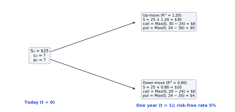
$S_{0} = 25$ ; after one year $S_{1}^{u} = 30$ ( $R^{u} = 1.20$ ) or $S_{1}^{d} = 20$ ( $R^{d} = 0.80$ ); $X = 24$ ; $R_{f} = 5%$ .

Call: $c_{1}^{u} = 6$ and $c_{1}^{d} = 0$ , so $h = 6/ (30 - 20) = 0.60$ . $V_{1} = 0.60 (30) - 6 = 12 = 0.60 (20)$ . $V_{0} = 12/1.05 = 11.429$ . $c_{0} = 0.60 (25) - 11.429 = 3.57$ .

Put: $p_{1}^{u} = 0$ and $p_{1}^{d} = 4$ , so $h = 4/10 = 0.40$ . $V_{1} = 0.40 (30) + 0 = 12 = 0.40 (20) + 4$ . $V_{0} = 11.429$ . $p_{0} = 11.429 - 0.40 (25) = 1.43$ .

Check with put–call parity: $c_{0} - p_{0} = 3.57 - 1.43 = 2.14 = 25 - 24/1.05$ .

The hedge portfolio is a pricing device; no cash needs to change hands to form it. Practical models split the option's life into many short periods, which gives many possible prices at expiration; the one-period tree shows the method.

Common exam traps

Discounting the hedge ratio, or compounding it, at the risk-free rate. $h$ is a pure ratio of payoff range to price range.
Using a short put in the put hedge (the put hedge is long put + long shares).

LOS 79.b — Risk neutrality

Because the hedged portfolio is riskless, option value does not depend on investors' risk preferences. The option can therefore be valued as if investors were risk-neutral: weight the two payoffs by risk-neutral probabilities, then discount that expected payoff using the risk-free rate.

Key concept

π_{U} = \frac{1 + R _{f} - R ^{d}}{R ^{u} - R ^{d}}, π_{D} = 1 - π_{U}

c_{0} = \frac{π _{U} c _{1}^{u} + π _{D} c _{1}^{d}}{1 + R _{f}}, p_{0} = \frac{π _{U} p _{1}^{u} + π _{D} p _{1}^{d}}{1 + R _{f}}

The steps: (1) compute the option payoffs after the up- and down-move; (2) take their probability-weighted average using $π_{U}$ and $π_{D}$ ; (3) discount one period at the risk-free rate.

Trees are often built with the down-move factor equal to the reciprocal of the up-move factor ( $R^{d} = 1/ R^{u}$ ), so an up-move of 1.25 pairs with a down-move of 0.80.

At Level I the risk-neutral probabilities are typically given; what matters is using them to weight the payoffs and discounting at the risk-free rate. $π_{U}$ and $π_{D}$ are pseudo-probabilities. They are not the actual probabilities of the moves; they come from the no-arbitrage hedge, which is why discounting at the risk-free rate is correct. In the example above, $π_{U} = (1.05 - 0.80) / (1.20 - 0.80) = 0.625$ , so $c_{0} = 0.625 \times 6/1.05 = 3.57$ , the same value as the hedge approach gives.

The name comes from what these probabilities do to the underlying. Weighted by $π_{U}$ and $π_{D}$ , the underlying's expected return equals the risk-free rate: $π_{U} R^{u} + π_{D} R^{d} = 1 + R_{f}$ . In the example, $0.625 \times 30 + 0.375 \times 20 = 26.25 = 25 \times 1.05$ : under these probabilities the share is expected to earn exactly the 5% risk-free rate.

Worked example: valuing a put both ways

A share trades at 40. Over one year it will either rise by a factor of 1.25 or fall by a factor of 0.80, and the 1-year risk-free rate is 3%. Value a 1-year European put with an exercise price of 42 using risk-neutral probabilities, and confirm the value with the hedge approach.

Step 1. End-of-year prices: $40 \times 1.25 = 50$ and $40 \times 0.80 = 32$ . Put payoffs: $p_{1}^{u} = 0$ and $p_{1}^{d} = 42 - 32 = 10$ .

Step 2. $π_{U} = (1.03 - 0.80) / (1.25 - 0.80) = 0.23/0.45 = 0.5111$ and $π_{D} = 1 - 0.5111 = 0.4889$ .

Step 3. $p_{0} = (0.5111 \times 0 + 0.4889 \times 10) /1.03 = 4.889/1.03 = 4.75$ .

Step 4. Hedge check: $h = (10 - 0) / (50 - 32) = 0.5556$ . The portfolio of 0.5556 shares and one put is worth $0.5556 \times 50 + 0 = 27.78$ after an up-move and $0.5556 \times 32 + 10 = 27.78$ after a down-move.

Step 5. $V_{0} = 27.78/1.03 = 26.97$ , so $p_{0} = 26.97 - 0.5556 \times 40 = 26.97 - 22.22 = 4.75$ .

Result. Both approaches value the put at 4.75.

Approach	Uses	Discount rate
Hedge (replication) portfolio	hedge ratio $h$ , certain end value	risk-free
Risk-neutral valuation	$π_{U}$ , $π_{D}$ from move sizes and $R_{f}$	risk-free

Common exam traps

Weighting payoffs by actual (real-world) probabilities.
Forgetting to discount the expected payoff. For the call in the example, this gives 3.75 instead of 3.57.
Discounting at a risk-adjusted rate instead of the risk-free rate.

Exam shortcuts

For European options with the same exercise price and expiration on an underlying with no income or holding costs, once the call is valued the put follows from put–call parity, $p_{0} = c_{0} - S_{0} + X / (1 + R_{f})$ , with no second hedge calculation.

Bottom line

A one-period binomial model values an option from the current underlying price, the exercise price, the up-move and down-move factors and the risk-free rate; it needs neither real-world probabilities nor a risk-adjusted discount rate.
For a call, the hedge portfolio is long $h$ shares and short one call, with $h = (c_{1}^{u} - c_{1}^{d}) / (S_{1}^{u} - S_{1}^{d})$ ; its certain end value is discounted at the risk-free rate and $c_{0} = h S_{0} - V_{0}$ .
For a put, the hedge portfolio is long $h$ shares and long one put, with $h = (p_{1}^{d} - p_{1}^{u}) / (S_{1}^{u} - S_{1}^{d})$ and $p_{0} = V_{0} - h S_{0}$ .
$π_{U} = (1 + R_{f} - R^{d}) / (R^{u} - R^{d})$ and $π_{D} = 1 - π_{U}$ , and an option's value is its payoffs weighted by $π_{U}$ and $π_{D}$ and discounted one period at the risk-free rate.
Risk-neutral probabilities are pseudo-probabilities derived from the no-arbitrage hedge, under which the underlying's expected return equals the risk-free rate; they are not the actual probabilities of the moves.
The hedge approach and risk-neutral valuation both discount at the risk-free rate and give the same option value.

Quick check

Question 1Core

Shares of Solvay Ridge follow the one-period binomial tree shown below. The one-year risk-free rate is 4%.

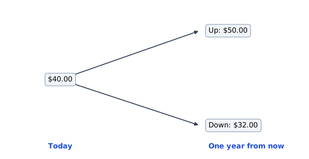
One-period binomial tree for Solvay Ridge shares

An analyst wants to write one-year European calls on the shares with an exercise price of $44 and hold shares so that the combined position has the same value at expiration whatever the share price. The number of shares to hold per call written is closest to:

Show answer and explanation

Correct answer: B

The hedge ratio equals the spread of the call's payoffs divided by the spread of the share prices. It is a ratio of payoffs, so no discounting or compounding at the risk-free rate is involved.

Call payoffs: $c_{1}^{u} = max (0, 50 - 44) = 6$ ; $c_{1}^{d} = max (0, 32 - 44) = 0$ .

h = \frac{c _{1}^{u} - c _{1}^{d}}{S _{1}^{u} - S _{1}^{d}} = \frac{6 - 0}{50 - 32} = \frac{6}{18} = 0.333

Check: up-move value $= 0.333 (50) - 6 = 10.67$ ; down-move value $= 0.333 (32) - 0 = 10.67$ . The portfolio of 0.333 shares per short call is worth 10.67 in both states.

Why the other options are wrong

A. 0.32 divides the hedge ratio by 1.04 ( $0.3333/1.04 = 0.3205$ ); the risk-free rate is used to value the portfolio and plays no part in computing $h$ .
C. 0.35 multiplies the hedge ratio by 1.04 ( $0.3333 \times 1.04 = 0.3467$ ); again, $h$ is not adjusted for interest.

Key takeaway $h = (c_{1}^{u} - c_{1}^{d}) / (S_{1}^{u} - S_{1}^{d})$ . The risk-free rate enters only when the certain portfolio value is discounted.

Practice Questions

Question 2Core

Shares of Keswick Marine trade at $60. In one year they will be worth either $78 after an up-move or $51 after a down-move. The one-year risk-free rate is 3%, and the risk-neutral probability of an up-move is 0.40. An analyst estimates the actual probability of an up-move at 0.55. Using risk-neutral valuation, the value of a one-year European call on the shares with an exercise price of $65 is closest to:

Show answer and explanation

Correct answer: A

Risk-neutral valuation weights the option's payoffs by the risk-neutral (pseudo-)probabilities and then discounts the expected payoff one period at the risk-free rate. The analyst's estimate of the actual probability of an up-move plays no role.

Payoffs at expiration: $c_{1}^{u} = max (0, 78 - 65) = 13$ ; $c_{1}^{d} = max (0, 51 - 65) = 0$ .

Risk-neutral probabilities: $π_{U} = 0.40$ , $π_{D} = 1 - 0.40 = 0.60$ .

Expected payoff: $0.40 (13) + 0.60 (0) = 5.20$

c_{0} = \frac{π _{U} c _{1}^{u} + π _{D} c _{1}^{d}}{1 + R _{f}} = \frac{5.20}{1.03} = 5.049 \approx $5.05

Check with the hedge approach: $h = 13/ (78 - 51) = 0.4815$ ; $V_{1} = 0.4815 (51) = 24.56$ ; $V_{0} = 24.56/1.03 = 23.84$ ; $c_{0} = 0.4815 (60) - 23.84 = 5.05$ . (The given probability is consistent with the tree: $(1.03 - 0.85) / (1.30 - 0.85) = 0.40$ .)

Why the other options are wrong

B. $5.20 is the risk-neutral expected payoff $0.40 \times 13$ without discounting it one year at the risk-free rate.
C. $6.94 weights the payoff by the analyst's actual probability instead of the risk-neutral probability: $0.55 \times 13/1.03$ .

Key takeaway Risk-neutral value = expected payoff using risk-neutral (not actual) probabilities, discounted at the risk-free rate.

Question 3Core

In a one-period binomial model, a call is valued by combining one short call with $h$ shares of the underlying so that the portfolio's value at the end of the period is the same after an up-move or a down-move. Rearranging this relationship, a position that replicates a long call consists of:

Show answer and explanation

Correct answer: C

The hedge portfolio is worth $V_{0} = h S_{0} - c_{0}$ , and because its end-of-period value is certain, $V_{0}$ is the present value of a riskless amount. Rearranged, $c_{0} = h S_{0} - V_{0}$ : the call is equivalent to owning $h$ shares while owing the riskless amount $V_{0}$ , that is, buying the shares partly with money borrowed at the risk-free rate. This leveraged long position in the underlying has the same payoff as the call in both states: 4 after an up-move and 0 after a down-move in the illustration below.

Illustration. $S_{0} = 30$ ; $S_{1}^{u} = 36$ , $S_{1}^{d} = 25$ ; $X = 32$ ; risk-free rate 3% for the period.

$c_{1}^{u} = 4$ , $c_{1}^{d} = 0$ , so $h = 4/ (36 - 25) = 0.3636$ .

Riskless value of the hedge: $V_{1} = 0.3636 \times 25 = 9.091$ , so $V_{0} = 9.091/1.03 = 8.826$ .

$c_{0} = 0.3636 \times 30 - 8.826 = 10.909 - 8.826 = 2.083$ .

Replication: buy 0.3636 shares for 10.909 and borrow 8.826. Up-move: $0.3636 \times 36 - 9.091 = 4$ . Down-move: $0.3636 \times 25 - 9.091 = 0$ . These are the call's payoffs.

Why the other options are wrong

A. Lending adds a riskless positive amount to the share position, so the portfolio would be worth more than the call after either move. In the hedge, $V_{0} = h S_{0} - c_{0}$ is the present value of a positive riskless amount, and $c_{0} = h S_{0} - V_{0}$ shows that the replicating portfolio owes that amount: it borrows.
B. Short shares plus lending gains when the price falls. That combination replicates a put: $p_{0} = V_{0} - h S_{0}$ .

Key takeaway In a one-period binomial model, a call can be replicated by buying $h$ shares with partly borrowed money, and a put by selling $h$ shares short and lending at the risk-free rate.

This reading has 8 questions in the full bank. Practice all of them.

Key Takeaways

$h = (c_{1}^{u} - c_{1}^{d}) / (S_{1}^{u} - S_{1}^{d})$ . The risk-free rate enters only when the certain portfolio value is discounted.
Risk-neutral value = expected payoff using risk-neutral (not actual) probabilities, discounted at the risk-free rate.
In a one-period binomial model, a call can be replicated by buying $h$ shares with partly borrowed money, and a put by selling $h$ shares short and lending at the risk-free rate.

What you'll learn

Binomial Model for Option Values

LOS 79.a — One-period binomial model: the hedge (replication) approach

Call: long h shares, short one call

Put: long h shares, long one put

LOS 79.b — Risk neutrality

Worked example: valuing a put both ways

Exam shortcuts

Bottom line

Practice Questions

Key Takeaways

Call: long $h$ shares, short one call

Put: long $h$ shares, long one put