Portfolio Construction · Reading 87

Modern Portfolio Theory

CFA Level I · Portfolio Construction · Reading 87: Portfolio Risk and Return: Part I · about 55 min

Portfolio Construction notes as a PDF78 pages · 1.2 MB · free, no sign-up · All PDFs

What you'll learn

LOS 87.a Describe the major asset classes (small- and large-cap stocks, corporate and government bonds, T-bills), their historical risk–return tradeoff, non-normal returns and liquidity.
LOS 87.b Explain risk aversion (versus risk neutrality and risk seeking) and what it implies for choosing among portfolios.
LOS 87.c Explain how an investor's utility function and indifference curves, combined with the capital allocation line, determine her optimal portfolio.
LOS 87.d Calculate and interpret the mean, variance, covariance and correlation of asset returns from historical data.
LOS 87.e Calculate and interpret the variance and standard deviation of a two-asset portfolio.
LOS 87.f Describe how combining assets whose returns are less than perfectly correlated reduces portfolio risk.
LOS 87.g Describe and interpret the minimum-variance frontier, the efficient frontier and the global minimum-variance portfolio.

Module 87.1

Historical Risk and Return

This reading describes the risk and return history of the major asset classes and explains risk aversion, utility, indifference curves, the capital allocation line and the choice of an optimal portfolio. It shows how to calculate mean, variance, covariance and correlation from historical returns and the standard deviation of a two-asset portfolio, how correlation drives diversification, and how the minimum-variance frontier, the global minimum-variance portfolio and the efficient frontier are defined.

LOS 87.a — Characteristics of the major asset classes

Portfolio construction starts with the asset classes an investor can combine. The classic building blocks are small-capitalization stocks, large-capitalization stocks, long-term corporate bonds, long-term government bonds (Treasury bonds) and Treasury bills (T-bills).

Risk and return go together

Long histories of market data (US data from 1926 onward, and similar data for other markets around the world) show a clear risk–return tradeoff: the asset classes with the highest average annual returns also have the highest standard deviation of returns.

Key concept

US asset class, 1926–2017	Average annual return (geometric mean)	Standard deviation (annualized monthly)
Small-cap stocks	12.1%	31.7%
Large-cap stocks	10.2%	19.8%
Long-term corporate bonds	6.1%	8.3%
Long-term government bonds	5.5%	9.9%
Treasury bills	3.4%	3.1%
Inflation	2.9%	4.0%

The pattern holds broadly rather than pair by pair: over this period long-term government bonds were slightly more volatile than long-term corporate bonds while earning a little less.

Over long periods, equities have earned higher average returns than fixed-income securities, but with a higher standard deviation of returns. Small-cap stocks have had the highest average return and the highest standard deviation, and T-bills the lowest of both.

Why the pattern makes sense

Theory predicts this pattern. Investors are risk averse, so they hold a riskier asset class only if they expect a higher average return as compensation for the extra risk (LOS 87.b).

Nominal versus real returns

Year-by-year nominal returns on US equities have swung widely, from losses above 40% to gains above 50%. Subtracting inflation gives an approximate real return. On the 1926–2017 figures, T-bills earned a real return of only about $3.4% - 2.9% = 0.5%$ , while large-cap stocks earned about $10.2% - 2.9% = 7.3%$ . Because inflation itself moved around a lot over the period, real returns have been more stable than nominal returns.

Example. Suppose a fund's nominal return last year was 9.0% and inflation was 3.5%. The approximate real return is $9.0% - 3.5% = 5.5%$ . If the same fund had returned 1.0% in a year of 6.0% inflation, its approximate real return would be $- 5.0%$ . Nominal returns can hide the effect of inflation.

Beyond mean and variance

Key concept

Describing an investment only by its expected return and variance (or standard deviation) is a simplification, because actual return distributions are not normal:

Negative skewness: returns show a tendency toward large downside surprises.
Excess kurtosis (fatter tails; kurtosis above 3): extreme outcomes, both up and down, happen more often than a normal distribution predicts.

These non-normal features (skewness $\neq = 0$ , kurtosis $\neq = 3$ ) should be considered when analyzing investments.

Liquidity is another characteristic. Illiquidity can depress a security's price and so raise its expected return. It matters most in emerging markets and for thinly traded securities, for example low-quality corporate bonds; developed-market government securities are highly liquid.

Common exam traps

An option giving equities a higher average return and a lower standard deviation than bonds contradicts the historical record.
Long-term government bonds are not the lowest-risk asset class: their prices move with interest rates, so they are more volatile than T-bills.
Negative skewness describes the shape of the distribution (a long left tail), not a negative average return.

Bottom line

Over long periods the asset classes with the highest average returns have also had the highest standard deviations, small-cap stocks being highest on both and T-bills lowest, although the pattern holds broadly and not for every pair.
Over long periods equities have earned higher average returns than fixed-income securities with a higher standard deviation, which fits risk-averse investors holding riskier asset classes only for a higher expected return.
The approximate real return is the nominal return minus inflation, and over 1926–2017 real returns were more stable than nominal returns because inflation itself varied a lot.
Return distributions are not normal: negative skewness means a tendency toward large downside surprises, and excess kurtosis (kurtosis above 3) means extreme outcomes occur more often than a normal distribution predicts.
Illiquidity can depress a security's price and so raise its expected return, which matters most in emerging markets and for thinly traded securities such as low-quality corporate bonds.

Quick check

Question 1Core

A pension trustee reviews close to a century of capital market history for the United States and other developed markets, comparing equity asset classes with fixed-income asset classes. Relative to fixed-income securities, equities have most likely shown:

Show answer and explanation

Correct answer: A

Long-run data show a positive risk–return tradeoff across asset classes. Both small-cap and large-cap stocks have earned higher average annual returns than long-term corporate and government bonds, and they have done so with a larger standard deviation of returns. Results in other developed markets are similar.

Why the other options are wrong

B. Equities have earned higher average returns than bonds over long periods. The extra return is the reward for their extra volatility.
C. Equities have been more volatile than bonds; higher return with lower risk would contradict the risk–return tradeoff.

Key takeaway Over long periods: more average return has come with more standard deviation (small caps > large caps > bonds > T-bills).

Module 87.2

Risk Aversion

LOS 87.b — Risk aversion and portfolio selection

A risk-averse investor dislikes risk: given two investments with the same expected return, she chooses the one with the lower risk (standard deviation). She will hold riskier assets if the extra expected return is adequate compensation for the extra risk. Financial models assume investors are risk averse, and the market prices of financial assets reflect the preferences of risk-averse investors, so riskier assets must offer higher expected returns.

Key concept

Investor type	Choice between two investments with equal expected return
Risk averse	Picks the less risky one
Risk neutral	Indifferent (cares only about expected return)
Risk seeking (risk loving)	Picks the riskier one

Illustration. A game pays $200 or $0 with equal probability (expected payoff $100). A risk-averse investor prefers a sure $100 to the game; a risk-seeking investor prefers the game; a risk-neutral investor is indifferent.

Dominance. A risk-averse investor never picks a portfolio that is beaten on both counts, that is, when another available portfolio has a higher (or equal) expected return and lower (or equal) risk, with at least one strictly better. Between a low-return/low-risk portfolio and a high-return/high-risk one, either can be a rational choice; which one depends on the investor's degree of risk aversion.

LOS 87.c — Utility, indifference curves and the optimal portfolio

Utility function

An investor's utility function expresses her trade-off between risk and return:

Key concept

U = E (r) - \frac{1}{2} A σ^{2}

where $E (r)$ is expected return and $σ^{2}$ the variance of returns (both in decimals), and $A$ is the investor's degree of risk aversion, also called the risk aversion coefficient. The larger $A$ , the more utility the investor gives up for each unit of variance. A risk-averse investor has $A > 0$ , a risk-neutral investor $A = 0$ and a risk-seeking investor $A < 0$ .

Example. With $A = 2$ , a portfolio with $E (r) = 8%$ and $σ = 10%$ gives $U = 0.08 - 0.5 \times 2 \times 0.1 0^{2} = 0.08 - 0.01 = 0.07$ .

Two results follow directly from the formula. A risk-free asset has $σ = 0$ , so its utility equals its return for every investor, whatever the value of $A$ . A risky portfolio, by contrast, is worth less to a more risk-averse investor: with the same 8% and 10%, an investor with $A = 6$ gets $U = 0.08 - 0.03 = 0.05$ , below the 0.07 of the investor with $A = 2$ .

Indifference curves

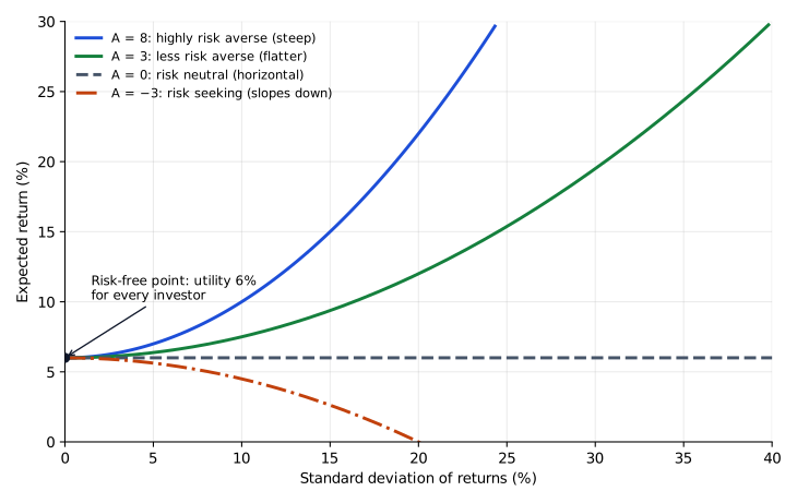
An indifference curve plots the risk–return combinations that give an investor the same expected utility. Drawing the curves from expected return and standard deviation alone assumes that these two are the only portfolio characteristics the investor cares about. For a risk-averse investor the curves slope upward (more risk must be paid for with more expected return) and curves higher up and to the left give more utility.

A more risk-averse investor needs more extra return per unit of extra risk, so her indifference curves are steeper (a higher $A$ ).
A less risk-averse investor has flatter indifference curves.

Solving the utility function for expected return gives $E (r) = U + \frac{1}{2} A σ^{2}$ , so the slope follows the sign of $A$ : upward when $A > 0$ , flat when $A = 0$ (risk neutral) and downward when $A < 0$ (risk seeking). The figure draws each kind with the same utility of 6%.

Expected return (0% to 30%) against standard deviation (0% to 40%). Four curves all start at an expected return of 6% with zero risk, the risk-free point where utility is 6% for every investor. A = 8 (highly risk averse) rises steeply: 10% expected return at 10% standard deviation and 22% at 20%. A = 3 (less risk averse) rises more gently: 7.5% at 10% and 12% at 20%. A = 0 (risk neutral) is a horizontal line at 6%. A = -3 (risk seeking) slopes down: 4.5% at 10% and 0% at 20%. — Indifference curves with a utility of 6% for investors with different risk aversion coefficients (illustrative numbers)

Adding the risk-free asset: the capital allocation line

Combine a risky portfolio (weight $w$ ) with a risk-free asset (weight $1 - w$ ). The risk-free asset's standard deviation is zero, and so is its correlation with the risky portfolio. In the two-asset portfolio formulas (LOS 87.e), every term involving the risk-free asset's risk therefore drops out, leaving

Key concept

E (R_{p}) = w E (R_{r i s k y}) + (1 - w) R_{f} σ_{p} = w σ_{r i s k y}

Portfolio risk is just the fraction $w$ of the risky portfolio's risk, so all combinations lie on a straight line. The line from the risk-free rate through the optimal risky portfolio is the capital allocation line (CAL). $w > 1$ means borrowing at the risk-free rate to invest more than 100% of equity in the risky portfolio (a leveraged position, beyond the risky portfolio on the CAL).

The two-fund separation theorem says that every investor's optimal portfolio is some combination of the same two "funds": the optimal risky portfolio and the risk-free asset. Investors differ only in how much they put in each.

Example. $R_{f} = 2%$ ; optimal risky portfolio $E (R) = 10%$ , $σ = 20%$ . With 30% in the risky portfolio: $E (R_{p}) = 0.30 (10%) + 0.70 (2%) = 4.4%$ and $σ_{p} = 0.30 \times 20% = 6%$ .

Choosing the optimal portfolio

The investor's optimal portfolio is the attainable portfolio that gives her the highest utility: the point where her highest attainable indifference curve is tangent to the CAL. With risky assets only, the tangency is with the efficient frontier, the set of risky portfolios with the highest expected return for each level of risk (LOS 87.g). Curves above it cannot be reached; curves below it are reachable but give less utility. The optimal portfolio is therefore not simply the one with the highest return, and it differs across investors because their indifference curves differ.

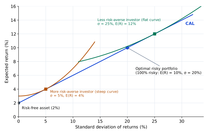
Graph of expected return (%) against standard deviation (%). The capital allocation line starts at the risk-free asset (0%, 2%) and passes through the optimal risky portfolio (standard deviation 20%, expected return 10%), continuing beyond it (borrowing). A steep indifference curve of a more risk-averse investor is tangent to the line at standard deviation 5% and expected return 4% (25% in the risky portfolio). A flat indifference curve of a less risk-averse investor is tangent at standard deviation 25% and expected return 12% (125% in the risky portfolio, financed by borrowing). — Capital allocation line and the optimal portfolios of two investors

The steep-curve (more risk-averse) investor is tangent near the risk-free end of the CAL: mostly T-bills, with low risk and low expected return. The flat-curve (less risk-averse) investor is tangent further out, with more in the risky portfolio (possibly borrowing) and higher risk and higher expected return.

Common exam traps

Risk aversion does not mean always choosing the least risky asset; it means choosing the less risky of two assets with the same expected return.
Do not reverse the slopes: a steep curve belongs to the more risk-averse investor, a flat curve to the less risk-averse one.
A leveraged investor (more than 100% in the risky portfolio) can still be risk averse, only less so, with flatter curves.
The line joining the risk-free asset and a risky portfolio is the capital allocation line; the capital market line is the special case where the risky portfolio is the market portfolio (Reading 88).
The optimum is the tangency with the highest attainable indifference curve. The lowest curve, or any point where a curve crosses the frontier, is wrong.
In the utility formula, enter returns and standard deviations as decimals (0.08, not 8) and keep the $\frac{1}{2}$ . With A = 2, $E (r) = 8%$ and $σ = 10%$ , dropping the $\frac{1}{2}$ gives 0.06 and entering 8 and 10 gives −92, instead of 0.07.

Exam shortcuts

A risk-free asset has $σ = 0$ , so its utility equals its return for every investor whatever the value of A, and no utility calculation is needed to rank it.

Bottom line

Given two investments with the same expected return, a risk-averse investor picks the less risky one, a risk-neutral investor is indifferent and a risk-seeking investor picks the riskier one.
Utility is $U = E (r) - \frac{1}{2} A σ^{2}$ with returns in decimals, where A is positive for a risk-averse investor, zero for a risk-neutral one and negative for a risk seeker, and a risky portfolio is worth less to a more risk-averse investor.
An indifference curve joins risk-return combinations with the same expected utility; for a risk-averse investor it slopes upward, a more risk-averse investor has steeper curves, and curves higher and to the left give more utility.
Combining a risky portfolio with the risk-free asset gives $E (R_{p}) = w E (R_{r i s k y}) + (1 - w) R_{f}$ and $σ_{p} = w σ_{r i s k y}$ , a straight capital allocation line, with $w > 1$ meaning borrowing at the risk-free rate.
Under two-fund separation every investor's optimal portfolio combines the same optimal risky portfolio with the risk-free asset, and investors differ only in how much they put in each.
The optimal portfolio is where the investor's highest attainable indifference curve is tangent to the CAL, or to the efficient frontier when only risky assets are available, so a more risk-averse investor sits nearer the risk-free end.

Quick check

Question 2Core

Priya Nair and Tomas Ekberg share the same capital market expectations. Ekberg's risk–return indifference curves are flatter than Nair's. Compared with Nair, Ekberg is most likely:

Show answer and explanation

Correct answer: A

Flatter indifference curves mean Ekberg requires less extra expected return for each additional unit of risk, so he is less risk averse than Nair. Facing the same set of portfolios, his flatter curve is tangent further out along the frontier (or CAL), so his optimal portfolio has more risk and a higher expected return.

Why the other options are wrong

B. Flatter curves indicate lower risk aversion; a more risk-averse investor has steeper curves.
C. The degree of risk aversion is right, but a less risk-averse investor's tangency point lies further out, at a higher expected return.

Key takeaway Flatter curves mean less risk aversion and an optimal portfolio with more risk and higher expected return.

Module 87.3

Portfolio Standard Deviation

LOS 87.d — Mean, variance, covariance and correlation from historical data

One asset

The mean return is the average of the period returns. Variance and standard deviation measure how widely returns spread around that mean. They are the usual measures of investment risk.

σ^{2} = \frac{\sum _{t = 1}^{T} ( R _{t} - μ ) ^{2}}{T} (population) s^{2} = \frac{\sum _{t = 1}^{T} ( R _{t} - R ˉ ) ^{2}}{T - 1} (sample)

Historical returns are a sample, so the sample variance (divide by $T - 1$ ) is normally used. Standard deviation is the square root of variance.

Two assets: covariance

Covariance measures how two variables move together over time.

Cov_{1, 2} = \frac{\sum _{t = 1}^{T} ( R _{1, t} - R ˉ _{1} ) ( R _{2, t} - R ˉ _{2} )}{T - 1}

Positive covariance: the returns tend to be above (or below) their means in the same periods, so they tend to move together.
Negative covariance: when one return is above its mean, the other tends to be below its mean. It does not mean they always move in opposite directions.
Zero covariance: no linear relationship, so knowing one return says nothing about the other in a linear sense.

Covariance is an absolute measure in squared return units. Its size depends on the assets' volatilities, so on its own it says little about the strength of the relationship.

Correlation

Standardizing covariance by the two standard deviations gives the correlation coefficient:

Key concept

ρ_{1, 2} = \frac{Cov _{1, 2}}{σ _{1} σ _{2}} ⟺ Cov_{1, 2} = ρ_{1, 2} σ_{1} σ_{2}

Correlation has no units and always lies between −1 and +1.

Key concept

Correlation	Meaning
$ρ = + 1$	Perfectly positively correlated: deviations from the means are always proportional and in the same direction
$ρ = - 1$	Perfectly negatively correlated: deviations always proportional and in opposite directions
$ρ = 0$	Uncorrelated: no linear relationship

Example. Three annual returns: Asset A 4%, 10%, 1%; Asset B 6%, 12%, 0%.

Means: $R ˉ_{A} = 15/3 = 5%$ , $R ˉ_{B} = 18/3 = 6%$ .
Deviations: A $- 1, + 5, - 4$ ; B $0, + 6, - 6$ .
$s_{A}^{2} = (1 + 25 + 16) /2 = 21$ , so $s_{A} = 4.58%$ ; $s_{B}^{2} = (0 + 36 + 36) /2 = 36$ , so $s_{B} = 6%$ .
$Cov_{A, B} = [(- 1) (0) + (5) (6) + (- 4) (- 6)] /2 = 54/2 = 27$ (in %²).
$ρ_{A, B} = 27/ (4.58 \times 6) = 0.98$ .

LOS 87.e — Portfolio standard deviation

For a two-asset portfolio with weights $w_{1}$ and $w_{2} = 1 - w_{1}$ :

E (R_{p}) = w_{1} E (R_{1}) + w_{2} E (R_{2})

Key concept

σ_{p}^{2} = w_{1}^{2} σ_{1}^{2} + w_{2}^{2} σ_{2}^{2} + 2 w_{1} w_{2} Cov_{1, 2} = w_{1}^{2} σ_{1}^{2} + w_{2}^{2} σ_{2}^{2} + 2 w_{1} w_{2} ρ_{1, 2} σ_{1} σ_{2}

σ_{p} = σ_{p}^{2}

The inputs are the weights, each asset's standard deviation (or variance) and the covariance (or correlation). Expected returns are needed for $E (R_{p})$ but not for $σ_{p}$ . Beta, which measures an asset's systematic risk relative to the market (Reading 88), is not an input.

Example. 60% in an equity fund ( $σ = 18%$ ) and 40% in a bond fund ( $σ = 10%$ ), $ρ = 0.20$ :

σ_{p}^{2} = 0.36 (0.0324) + 0.16 (0.0100) + 2 (0.6) (0.4) (0.2) (0.18) (0.10) = 0.011664 + 0.0016 + 0.001728 = 0.014992

$σ_{p} = 0.014992 = 12.24%$ . With $ρ = + 1$ the answer would be the weighted average $0.6 (18%) + 0.4 (10%) = 14.8%$ .

Common exam traps

When variances are given, take square roots before dividing the covariance by $σ_{1} σ_{2}$ .
Correlation outside −1 to +1 means an arithmetic error (e.g., dividing the wrong way).
Sample statistics divide by $T - 1$ , not $T$ . Dividing by T = 3 in the three-year example gives a variance of 14 for Asset A and a covariance of 18 instead of 21 and 27.
Portfolio variance or standard deviation: read which one is asked.
Square the weights and the standard deviations (in decimals) in the first two terms, and keep the factor 2 on the covariance term. In the 60/40 example, dropping the 2 gives 11.89% and leaving the weights unsquared gives 15.86%, instead of 12.24%.

Bottom line

Historical returns are a sample, so the sample variance divides the squared deviations by $T - 1$ , and the standard deviation is its square root.
Covariance measures how two returns move together: positive when they tend to be above or below their means in the same periods, negative when one tends to be above its mean while the other is below, and zero when there is no linear relationship.
Covariance is in squared return units and depends on the assets' volatilities, whereas the correlation $ρ_{1, 2} = Cov_{1, 2} / (σ_{1} σ_{2})$ has no units and lies between −1 and +1.
Two-asset portfolio variance is $w_{1}^{2} σ_{1}^{2} + w_{2}^{2} σ_{2}^{2} + 2 w_{1} w_{2} ρ_{1, 2} σ_{1} σ_{2}$ , so its inputs are the weights, the standard deviations and the covariance or correlation, with expected returns and beta not needed for $σ_{p}$ .

Quick check

Question 3Core

An analyst collects four years of returns for two stocks:

Annual returns on two stocks (%)

Year	Stock P	Stock Q
1	9	14
2	3	6
3	12	10
4	8	10

Using the sample formula, the covariance between the returns of Stock P and Stock Q (in percent squared) is closest to:

Show answer and explanation

Correct answer: A

Sample covariance is the sum of the products of the two stocks' deviations from their own means, divided by $T - 1$ . The products sum to 24 over four observations, so the covariance is $24/3 = 8$ .

Means: $R ˉ_{P} = (9 + 3 + 12 + 8) /4 = 8%$ ; $R ˉ_{Q} = (14 + 6 + 10 + 10) /4 = 10%$

Year	$R_{P} - R ˉ_{P}$	$R_{Q} - R ˉ_{Q}$	Product
1	1	4	4
2	−5	−4	20
3	4	0	0
4	0	0	0

Cov_{P, Q} = \frac{4 + 20 + 0 + 0}{4 - 1} = \frac{24}{3} = 8

Why the other options are wrong

B. 14 is the sample variance of Stock P $(1 + 25 + 16 + 0) /3$ . The question asks for the covariance between P and Q.
C. 24 is the sum of the cross-products before dividing by $T - 1 = 3$ .

Key takeaway Covariance: multiply paired deviations, sum, divide by $T - 1$ . Don't confuse it with one stock's variance.

Module 87.4

The Efficient Frontier

LOS 87.f — Investing in assets that are less than perfectly correlated

When $ρ_{1, 2} = + 1$ , the portfolio variance formula collapses to a perfect square:

σ_{p}^{2} = (w_{1} σ_{1} + w_{2} σ_{2})^{2} \Rightarrow σ_{p} = w_{1} σ_{1} + w_{2} σ_{2}

With perfect positive correlation, portfolio standard deviation is simply the weighted average of the assets' standard deviations: there is no diversification benefit. The lowest-risk (long-only) portfolio is then 100% in the asset with the lower standard deviation.

For any correlation below +1, the covariance term is smaller, so portfolio standard deviation is less than the weighted average of the individual standard deviations. That reduction is the diversification benefit, and the lower the correlation, the larger it is. At $ρ = 0$ the covariance term vanishes; for negative $ρ$ it becomes negative and cuts risk further. At $ρ = - 1$ the variance is again a perfect square, $(w_{1} σ_{1} - w_{2} σ_{2})^{2}$ , so $σ_{p} = ∣ w_{1} σ_{1} - w_{2} σ_{2} ∣$ . Choosing the weights so that $w_{1} σ_{1} = (1 - w_{1}) σ_{2}$ sets this to zero and gives a zero-variance portfolio:

Key concept

w_{1} = \frac{σ _{2}}{σ _{1} + σ _{2}}

With long positions only, a zero-variance portfolio of two risky assets is possible only when $ρ = - 1$ ; at $ρ = 0$ risk falls but cannot reach zero.

Example. Two assets with $σ_{1} = 16%$ , $σ_{2} = 24%$ , equally weighted:

Key concept

$ρ$	Portfolio variance	Portfolio $σ$
+1	0.0400	20.00%
+0.5	0.0304	17.44%
0	0.0208	14.42%
−0.5	0.0112	10.58%
−1	0.0016	4.00%

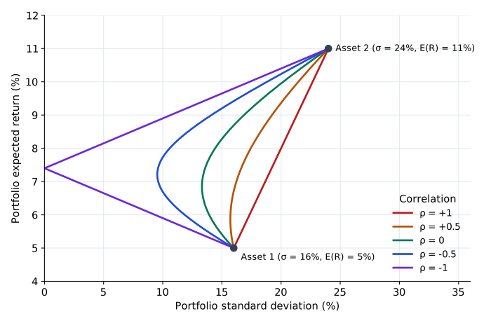
At $ρ = - 1$ the zero-variance mix is $w_{1} = 24/40 = 60%$ ; the equal-weighted mix still has 4.00% risk. The figure shows all long-only combinations of two assets ( $E (R_{1}) = 5%$ , $E (R_{2}) = 11%$ ) for several correlations. Correlation does not enter $E (R_{p}) = w_{1} E (R_{1}) + w_{2} E (R_{2})$ , so a given mix of weights has the same expected return on every curve. A lower correlation only cuts the risk of that mix, which is why the curve bulges further to the left. The $ρ = - 1$ curve reaches the vertical axis at $0.60 (5%) + 0.40 (11%) = 7.4%$ , the expected return of the zero-variance mix.

Graph of portfolio expected return (%) against portfolio standard deviation (%) for all long-only combinations of Asset 1 (standard deviation 16%, expected return 5%) and Asset 2 (standard deviation 24%, expected return 11%). For correlation +1 the combinations form a straight line between the two assets. For +0.5, 0 and -0.5 the curves bow increasingly to the left. For -1 the combinations form two straight lines meeting at zero standard deviation with an expected return of 7.4% (60% in Asset 1). — Two-asset portfolio risk and return for different correlations

Adding an asset. If a new asset has the same standard deviation as the existing portfolio and a correlation with it below +1, adding it reduces portfolio standard deviation. With equal risk and return, the candidate with the lowest covariance (correlation) with the portfolio reduces risk the most. For the same reason investors add other asset classes, such as bonds, real estate and foreign stocks, to their domestic stocks.

LOS 87.g — Minimum-variance frontier, efficient frontier and the global minimum-variance portfolio

For each level of expected return, the portfolio with the lowest standard deviation is a minimum-variance portfolio; together they form the minimum-variance frontier. The minimum-variance portfolio farthest to the left, which is the lowest-risk risky portfolio of all, is the global minimum-variance portfolio.

Key concept

Risk-averse investors want the highest expected return for each level of risk. The portfolios that offer it form the efficient frontier: the upper part of the minimum-variance frontier, starting at the global minimum-variance portfolio. Equivalently, an efficient portfolio is not dominated by any other attainable portfolio: no attainable portfolio offers a higher expected return with the same or lower risk. Efficient portfolios do not dominate one another, because moving along the frontier trades more risk for more expected return.

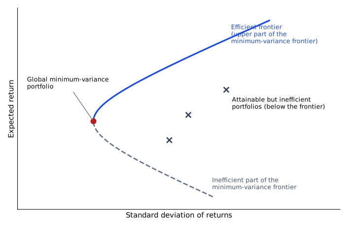
Minimum-variance frontier, efficient frontier and global minimum-variance portfolio

A portfolio below the efficient frontier is inefficient: another attainable portfolio offers a higher expected return for the same risk (or the same return with lower risk). Risk-averse investors will not choose it.
A portfolio above the efficient frontier is not attainable.
The frontier is concave: its slope decreases as risk increases (each extra unit of risk buys less extra return).
Lower correlations among assets move the frontier to the left (up and to the left, the "northwest"): the same returns with less risk.

Inputs (Markowitz). Risk is measured by the variance (standard deviation) of returns. Building the efficient frontier requires each security's expected return, variance and the covariances between all pairs of securities. Investors' risk aversion is not an input; it matters only when choosing a portfolio on the frontier (Module 87.2).

Spotting an inefficient portfolio. Portfolio K: $E (R) = 9%$ , $σ = 17%$ ; Portfolio L: $E (R) = 10%$ , $σ = 15%$ . L has the higher return and the lower risk, so K cannot be on the efficient frontier.

When investors can lend and borrow at a risk-free rate below the expected returns on the efficient frontier, they combine the risk-free asset with the optimal risky portfolio (two-fund separation). The capital allocation line touches the concave efficient frontier only at the optimal risky portfolio, so every other frontier portfolio, including the global minimum-variance portfolio, lies below the line and is not an optimal holding for a rational investor. That includes the frontier portfolios beyond the tangency point. For an investor who wants more expected return than the optimal risky portfolio offers, borrowing at the risk-free rate to move further out along the line gives a higher expected return for the same standard deviation.

Common exam traps

Efficient frontier = highest return for each level of risk. "Each level of risk tolerance" is a distractor.
A covariance equal to $σ_{1} σ_{2}$ signals $ρ = + 1$ , even when no correlation is quoted.
Diversification helps whenever $ρ < + 1$ , including positive correlations below +1.

Exam shortcuts

With $ρ = + 1$ , portfolio standard deviation is the weighted average of the assets' standard deviations, so the full variance formula is not needed.
A portfolio with a lower expected return and a higher standard deviation than another attainable portfolio is dominated, so it can be ruled out as efficient without plotting the frontier.

Bottom line

For any correlation below +1, portfolio standard deviation is less than the weighted average of the assets' standard deviations, and the lower the correlation, the larger this diversification benefit.
With long positions only, a zero-variance portfolio of two risky assets exists only when $ρ = - 1$ , with $w_{1} = σ_{2} / (σ_{1} + σ_{2})$ .
Correlation does not affect a portfolio's expected return, only its risk, so a lower correlation moves each mix of weights to the left at the same expected return.
Adding an asset with the same standard deviation as the portfolio and a correlation with it below +1 reduces portfolio risk, and among otherwise equal candidates the one with the lowest correlation reduces it most.
The efficient frontier is the upper part of the minimum-variance frontier starting at the global minimum-variance portfolio; portfolios below it are inefficient, portfolios above it are not attainable, and it is concave.
The Markowitz inputs are each security's expected return and variance and the covariances between all pairs, investors' risk aversion is not an input, and when investors can lend and borrow at a risk-free rate below the frontier's expected returns, the CAL touches the frontier only at the optimal risky portfolio.

Quick check

Question 4Core

Fund Lark has a standard deviation of returns of 7.4%, and Fund Wren has a standard deviation of returns of 5.2%. The two funds' returns are perfectly positively correlated. If short sales are not allowed, which allocation minimizes the standard deviation of a portfolio of the two funds?

Show answer and explanation

Correct answer: A

With a correlation of +1 there is no diversification benefit: portfolio standard deviation is just the weighted average of the two funds' standard deviations. The weighted average is lowest when everything is in the fund with the lower standard deviation, Wren (5.2%).

With $ρ = + 1$ : $σ_{p} = w_{L} (7.4%) + w_{W} (5.2%)$ , a weighted average that is minimized at $w_{W} = 100%$ , giving $σ_{p} = 5.2%$ .

Why the other options are wrong

B. Putting everything in Lark gives the highest possible portfolio risk (7.4%), because Lark is the more volatile fund.
C. These weights $(w_{L a r k} = 5.2/12.6 = 41%)$ would create a zero-risk portfolio only if the correlation were −1. With $ρ = + 1$ , this mix has $σ_{p} = 0.41 (7.4%) + 0.59 (5.2%) = 6.1%$ , more than Wren alone.

Key takeaway With perfect positive correlation, hold only the lower- $σ$ asset to minimize risk.

Practice Questions

Question 5Core

Investors can borrow and lend at the risk-free rate, which is below the expected return of every portfolio on the efficient frontier of risky assets, and all investors hold the same expectations about risky assets. A rational, risk-averse investor is least likely to choose which of the following as her entire portfolio?

Show answer and explanation

Correct answer: B

By the two-fund separation theorem, every investor's optimal portfolio is a combination of the risk-free asset and the optimal risky portfolio, so it lies on the capital allocation line (CAL). Because the risk-free rate is below the frontier's returns, the CAL touches the concave efficient frontier only at the optimal risky portfolio, which lies above the global minimum-variance portfolio; every other risky portfolio, including the global minimum-variance portfolio, plots below the CAL. A mix of the risk-free asset and the optimal risky portfolio with the same standard deviation offers a higher expected return, so the global minimum-variance portfolio is not an optimal choice.

Why the other options are wrong

A. A very risk-averse investor may rationally hold only the risk-free asset, the starting point of the capital allocation line.
C. A less risk-averse investor may rationally borrow to hold more than 100% of her equity in the optimal risky portfolio, a point on the line beyond the risky portfolio.

Key takeaway With a risk-free asset, optimal portfolios lie on the CAL through the optimal risky portfolio; the global minimum-variance portfolio lies below the CAL and is dominated.

This reading has 75 questions in the full bank. Practice all of them.

Key Takeaways

Over long periods: more average return has come with more standard deviation (small caps > large caps > bonds > T-bills).
Flatter curves mean less risk aversion and an optimal portfolio with more risk and higher expected return.
Covariance: multiply paired deviations, sum, divide by $T - 1$ . Don't confuse it with one stock's variance.
With perfect positive correlation, hold only the lower- $σ$ asset to minimize risk.
With a risk-free asset, optimal portfolios lie on the CAL through the optimal risky portfolio; the global minimum-variance portfolio lies below the CAL and is dominated.