Portfolio Construction · Reading 88
Systematic vs Unsystematic Risk
CFA Level I · Portfolio Construction · Reading 88: Portfolio Risk and Return: Part II · about 1 h 3 min
What you'll learn
- LOS 88.a Describe what happens to risk and expected return when a risk-free asset is combined with a portfolio of risky assets.
- LOS 88.b Explain the capital allocation line (CAL) and the capital market line (CML), including lending and borrowing portfolios and the market portfolio.
- LOS 88.c Explain systematic and nonsystematic risk and why nonsystematic risk earns no additional expected return.
- LOS 88.d Explain return generating models, including multifactor models and the market model, and their uses.
- LOS 88.e Calculate and interpret beta from covariance, correlation and standard deviations, or from the CAPM relation.
- LOS 88.f Explain the capital asset pricing model (CAPM), its assumptions, and the security market line (SML), and contrast the SML with the CML.
- LOS 88.g Calculate and interpret an asset's expected (required) return using the CAPM.
- LOS 88.h Describe and demonstrate applications of the CAPM and the SML, such as identifying undervalued and overvalued securities.
- LOS 88.i Calculate and interpret the Sharpe ratio, Treynor measure, M-squared and Jensen's alpha.
Module 88.1
Systematic Risk and Beta
This reading adds a risk-free asset to a risky portfolio to derive the capital allocation line and the capital market line, separates systematic from unsystematic risk, and covers return generating models, the market model and the calculation of beta. It then derives the CAPM and the security market line, shows how to calculate required returns and identify mispriced securities, and how to compute and interpret the Sharpe ratio, M-squared, the Treynor measure and Jensen's alpha.
LOS 88.a — Adding a risk-free asset to a risky portfolio
A risk-free asset has a standard deviation of returns of zero, and its returns have zero correlation with the returns of any risky asset. When an investor puts a weight in a risky portfolio P and in the risk-free asset, the two-asset portfolio formulas reduce to two simple expressions:
- The expected return is a weighted average of the risk-free rate and the risky portfolio's expected return.
- The standard deviation is the risky weight times the risky portfolio's standard deviation, because the risk-free asset contributes no variance and no covariance.
- Both and are linear in , so every combination plots on a straight line that starts at on the vertical axis and passes through P.
A single risky portfolio plus the risk-free asset therefore lets investors with very different degrees of risk aversion reach the level of risk they want. The resulting combinations can dominate risky portfolios that lie below the line.
Example. A risky fund has and ; .
| Weight in risky fund | Expected return | Standard deviation |
|---|---|---|
| 0.70 (lending 30%) | ||
| 1.00 | 9.0% | 15.0% |
| 1.25 (borrowing 25%) |
Common exam traps
- A 50/50 mix has exactly half the risky portfolio's standard deviation. Expecting diversification to push it lower is the mistake: the risk-free return never varies, so it cannot offset any of P's swings.
- The variance is not a weighted average of the variances. The standard deviation is a weighted average of the standard deviations (one of which is zero). For the 0.70 weight in the example, averaging the variances gives a standard deviation of 12.55% instead of 10.5%.
LOS 88.b — The capital allocation line (CAL) and the capital market line (CML)
The capital allocation line (CAL) is the line of risk–return combinations available from the risk-free asset and one particular risky portfolio. Each risky portfolio produces its own CAL. Of all the CALs, the investor should use the one whose set of portfolios she prefers most. That is the steepest line from , the one tangent to the efficient frontier, called the optimal CAL. The tangency point is the optimal risky portfolio: of all risky portfolios, it has the highest excess return per unit of standard deviation, , which is the Sharpe ratio of LOS 88.i. Because every CAL starts at , the optimal CAL offers a higher expected return than any other CAL at every level of risk above zero.
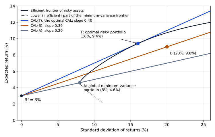
In the figure, . B has a higher expected return than the global minimum-variance portfolio A and a steeper CAL: against . T's CAL is steeper still, , so T is the optimal risky portfolio. B lies inside the frontier, and T offers both less risk and more expected return than B. The investor then picks the point on the optimal CAL that maximizes her expected utility, where her highest indifference curve touches the line.
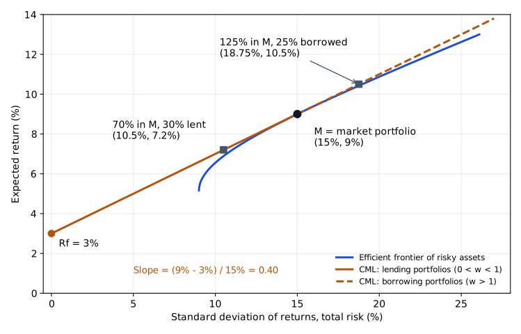
If investors had different forecasts, each would find a different tangency portfolio and a different CAL. Capital market theory assumes homogeneous expectations: everyone has the same estimates of expected returns, standard deviations and correlations. Everyone then faces the same efficient frontier and the same tangency portfolio, and that portfolio must be the market portfolio. The market portfolio is the portfolio of all risky assets in existence, held in market-value weights; it contains no risk-free asset. The common optimal CAL is called the capital market line (CML).
Key concept
- The intercept is . The slope, , is the excess return per unit of total risk (standard deviation). It equals the Sharpe ratio of the market portfolio.
- is the market risk premium. Writing the CML as shows that each unit of market risk an investor accepts adds one market risk premium to her expected return.
- Risk on the horizontal axis is standard deviation (total risk). Beta is the risk measure of the security market line (LOS 88.f).
- Points between and M are lending portfolios, with part of the money invested at . Points beyond M, further up the line, are borrowing portfolios: the investor borrows at and invests more than 100% of her equity in M (buying on margin). All portfolios on the CML hold the same risky portfolio (M), so their returns are perfectly positively correlated with each other and they carry no unsystematic risk.
Example. , , . Slope . A CML portfolio with has ; its weight in M is . The risk-free asset has a beta of 0 and M has a beta of 1, so the beta of any CML portfolio equals its weight in M: 0.80 here, and 1.25 for an investor who borrows a quarter of her equity and puts 125% of it in M.
Two-fund separation. Combining the CML with an investor's indifference curves splits portfolio choice into two separate decisions. Which risky assets to hold is the same decision for everyone: hold the market portfolio. How much risk to take, meaning how much to lend or borrow at , depends on the investor's own risk aversion. This is the two-fund separation theorem (the separation theorem): every investor's optimal portfolio combines just two funds, the risk-free asset and the optimal risky portfolio. Security selection thereby reduces to building one well-diversified portfolio.
Passive vs. active. Investors who believe market prices are informationally efficient follow a passive investment strategy. They hold an index fund as a proxy for M and split their money between it and the risk-free asset. Investors who think they can identify mispriced securities use active portfolio management, overweighting securities they consider undervalued and underweighting those they consider overvalued.
Common exam traps
- Calling the market portfolio "all stocks", or a mix of risky assets and the risk-free asset, is wrong; a broad equity index is only a proxy for it.
- The market portfolio is found by drawing a line from the risk-free rate tangent to the efficient frontier. A line from some other point on the return axis, or the point where an investor's indifference curve touches the frontier, does not locate it.
- Reading capital market theory as "everyone holds exactly M" is a mistake; only the risky part of each investor's portfolio is the same.
LOS 88.c — Systematic and unsystematic risk
Key concept
| Systematic risk | Unsystematic risk |
|---|---|
| Also called market risk or nondiversifiable risk | Also called unique risk, firm-specific risk or diversifiable risk |
| Caused by economy-wide factors (GDP growth, interest rates, inflation) | Caused by events specific to one company or industry |
| Cannot be removed by diversification | Falls as more (imperfectly correlated) securities are added |
| Priced: compensated with higher expected return | Not priced in equilibrium |
Total risk is measured by the standard deviation (or variance) of returns. Exam convention: total risk = systematic risk + unsystematic risk is stated as a simple sum, with total risk measured by standard deviation. Current practice: the sum is exact for variances, as in the market model ; the standard deviations of the two parts do not add up to the total standard deviation.
Systematic risk applies to single securities as well as to portfolios. Makers of luxury goods, such as sports cars and premium motorcycles, respond strongly to the business cycle and have high systematic risk. Utilities respond little to market-wide factors and have low systematic risk. As the number of randomly chosen stocks in a portfolio grows, total risk declines and approaches market risk. According to one study, about 12 to 18 stocks capture roughly 90% of the maximum diversification benefit; another put the number at about 30 stocks. Either figure is far smaller than the number of securities in the market.
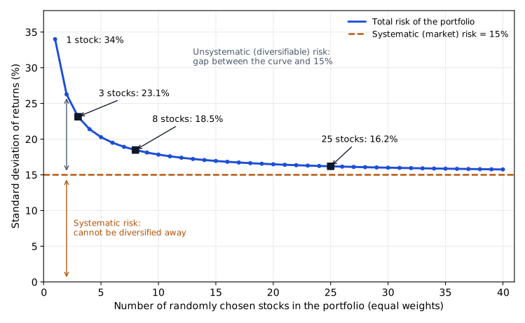
As unsystematic risk is diversified away, the portfolio behaves more and more like the market, so its correlation with the market moves toward +1. The market portfolio is perfectly diversified, and all of its risk is systematic.
Bonds. The same reasoning applies to a bond portfolio. A surprise that hits one issuer, such as a downgrade, can be diversified away by holding bonds of many issuers, while economy-wide changes, such as a recession or a rise in interest rates or inflation, affect all bonds and cannot be diversified away.
Why unsystematic risk earns no premium. Capital market theory assumes diversification is costless; a low-cost index fund comes close. Investors will not be paid for bearing a risk they could remove for free, so in equilibrium the expected (required) return depends only on systematic risk. A single-drug biotech stock can have very high total risk yet low systematic risk, and therefore a low equilibrium return. A steady machine-tool maker with modest total risk but high sensitivity to the business cycle requires a higher return. A portfolio of 50 or 100 such biotech stocks would carry little of that firm-specific uncertainty, because the successes and failures offset one another. A security's systematic risk is measured by what it contributes to the risk of a well-diversified portfolio.
Common exam traps
- Individual securities carry both systematic and unsystematic risk. Only well-diversified portfolios are (approximately) free of unsystematic risk.
- Adding randomly chosen stocks reduces unsystematic risk and leaves the expected level of systematic risk unchanged. Deliberately adding high-beta (low-beta) stocks does raise (lower) the portfolio's systematic risk.
- Rejecting total risk = systematic risk + unsystematic risk because standard deviations do not add is the mistake; under the exam convention above, that identity is the expected answer.
LOS 88.d — Return generating models and the market model
A return generating model estimates an asset's expected return from its exposure to one or more factors. Factors may be macroeconomic (GDP growth, inflation, consumer confidence), fundamental (earnings, earnings growth, firm size, research spending) or statistical. In practice, most models rely mainly on macroeconomic and fundamental factors. Statistical factors frequently lack any grounding in finance theory. They may capture a pattern specific to one sample period that was found by data mining (testing one data set over and over).
The multifactor model in excess-return form is:
Each is a factor sensitivity (factor loading). The first factor is often the market's excess return.
- The Fama and French model uses three factors: the market's excess return, firm size, and the book-to-market (book value to market value) ratio.
- Carhart adds a fourth factor, price momentum, based on prior-period returns. The four factors explain a good share of the differences in US equity returns over the period in which the model was estimated.
A single-factor model uses just one factor, whatever that factor is (for example, only the book-to-market ratio, or only the earnings growth rate). The single-factor model whose factor is the market's excess return is the single-index model: .
The market model is a simplified single-index model estimated by regressing the asset's return on the market's rate of return:
- and are estimated from historical returns. The expected return is .
- It is used to estimate and to measure abnormal return, : the actual return minus the return expected given the actual market return.
- For consistency with the single-index model, can be set to .
Example. A stock's market model is . The market returns 6%, so the expected return is . If the stock actually returned 8.5%, its abnormal return is .
Common exam traps
- The market model regresses on the market's rate of return (), not on its excess return or a risk-adjusted return.
- The number of factors decides "single-factor" versus "multifactor"; the type of factor does not.
LOS 88.e — Calculating and interpreting beta
Beta is a standardized measure of the covariance of an asset's return with the market's return. It measures systematic risk only:
Key concept
- The market's beta is 1, because the covariance of the market's return with itself is its variance: . The (value-weighted) average beta of all stocks is also 1. A beta of 0 means the asset's return is uncorrelated with the market. Negative betas are possible.
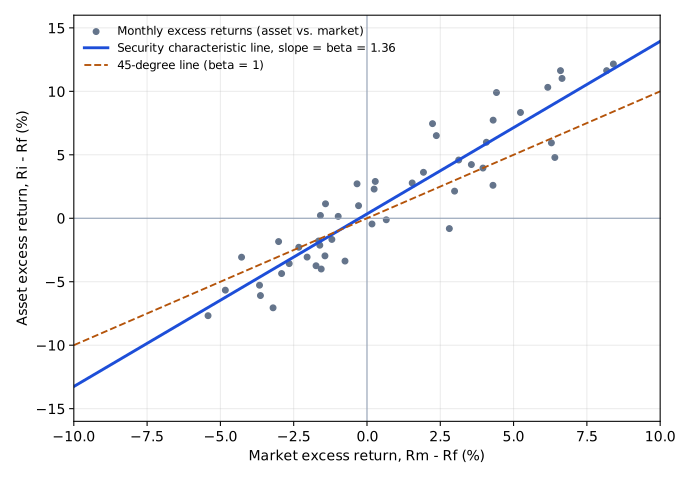
- In practice beta is estimated as the slope of a regression of the asset's excess returns on the market's excess returns. The least squares line, which minimizes the sum of squared vertical distances of the points from the line, is the security characteristic line. Its slope is . A slope steeper than 45° means : the asset's return reacts more strongly to systematic factors than the market's does.
Example. , , .
Covariance ; . Equivalently, .
Backing beta out of the CAPM. The CAPM (LOS 88.f) states . Rearranging it gives . If a stock is expected to earn 12% with and , .
Common exam traps
- Divide the covariance by the market variance. Dividing by the market standard deviation is a common mistake. In the example, dividing 0.01764 by 0.14 gives 0.126 instead of 0.90.
- When given variances, take square roots before using .
- The ratio is , the asset's standard deviation over the market's. Do not invert it, and do not forget to multiply by the correlation. In the example, inverting the ratio gives 0.225 and leaving out the correlation gives 2.0, instead of 0.90.
- When backing out beta, subtract from both the asset's and the market's expected return. In the example, 12/7 gives 1.71 and 10/7 gives 1.43 instead of 2.0.
Exam shortcuts
- The risk-free asset has a beta of 0 and the market portfolio a beta of 1, so the beta of any portfolio on the CML equals its weight in M, with no covariance calculation needed.
Bottom line
- Combining a risky portfolio P with the risk-free asset gives and , so every combination lies on a straight line from through P.
- The optimal CAL is the steepest line from , tangent to the efficient frontier at the optimal risky portfolio, which has the highest excess return per unit of standard deviation of all risky portfolios.
- Under homogeneous expectations every investor's tangency portfolio is the market portfolio of all risky assets in market-value weights, and the CML, , measures risk by standard deviation, with investors differing only in how much they lend or borrow at .
- Exam convention: total risk = systematic risk + unsystematic risk, with total risk measured by standard deviation; current practice: the sum is exact for variances only; in either case only systematic risk is priced, because capital market theory assumes unsystematic risk can be diversified away at no cost.
- The market model regresses an asset's return on the market's rate of return and gives the abnormal return , while multifactor models such as Fama and French (market, size, book-to-market) and Carhart (adding momentum) use several factors.
- Beta is , measures systematic risk only, and equals 1 for the market.
Quick check
An investor combines a risk-free asset with a portfolio of risky assets. Which statement about the new portfolio is least accurate?
Show answer and explanation
Correct answer: A
The variance of the new portfolio is , not . The standard deviation, rather than the variance, is the weighted average of the two assets' standard deviations (zero for the risk-free asset and for the risky portfolio).
Example with , : variance (standard deviation 10%), whereas a weighted average of variances would give (standard deviation 14.1%).
Why the other options are wrong
- B. Accurate: .
- C. Accurate: because the risk-free asset has zero standard deviation and zero correlation, .
Key takeaway Standard deviation is linear in the risky weight; variance is not.
Module 88.2
The CAPM and the SML
LOS 88.f — The CAPM, its assumptions, and the security market line (SML)
Only systematic risk is priced, so the relevant risk of any asset is its covariance with the market. Plotting expected return against , or against beta after standardizing by the market variance, gives the security market line (SML). The equation of the SML is the capital asset pricing model (CAPM):
The intercept is (beta 0), the market plots at , and the slope is the market risk premium . With a positive market risk premium, expected return rises linearly with systematic risk.
Assumptions of the CAPM
| Assumption | Meaning |
|---|---|
| Risk aversion | Investors demand a higher expected return to accept more risk |
| Utility maximizing investors | Rational investors each choose the risk–return combination that maximizes their own expected utility |
| Frictionless markets | No taxes, no transaction costs and no other impediments to trading |
| One-period horizon | All investors share the same single-period time horizon |
| Homogeneous expectations | All investors have the same estimates of expected returns, standard deviations and correlations |
| Divisible assets | All investments are infinitely divisible |
| Competitive markets | Investors are price takers; no single investor's trades can influence prices |
Comparing the CML and the SML
Key concept
| Capital market line (CML) | Security market line (SML) | |
|---|---|---|
| Risk measure (x-axis) | Standard deviation (total risk) | Beta (systematic risk) |
| What plots on it in equilibrium | Only efficient portfolios ( combined with M) | All properly priced securities and portfolios, diversified or not |
| Slope | ||
| Diversification of points on it | Always well diversified; only systematic risk | Can be single stocks or concentrated portfolios; any unsystematic risk they carry is not priced |
The two lines are drawn against different risk measures, so there is no point at which they "converge". In equilibrium an inefficient portfolio or a single stock plots below the CML but on the SML. Every asset with a beta of 1 plots at the same point on the SML as the market, whatever its total risk.
Common exam traps
- Picking the stock with the highest standard deviation as the one with the highest equilibrium return is the classic mistake; the CAPM prices beta only.
- Risk aversion does not require holding the risk-free asset. A risk-averse investor may still borrow to buy more of M.
- The security characteristic line (LOS 88.e) is not the SML. Its slope is one asset's beta, while the slope of the SML is the market risk premium.
LOS 88.g — Expected (required) return with the CAPM
Substitute the inputs into . Check whether the question gives the expected market return or the market risk premium .
Example. , , : . Because , the stock's expected return exceeds the market's.
Useful rearrangements and relationships:
- Market risk premium: . The same equation solved for beta is shown under LOS 88.e.
- Nominal risk-free rate real risk-free rate + expected inflation.
- With a positive market risk premium (), a negative beta gives a required return below . If , a negative beta gives a required return above . For example, with , and , the required return is .
- Holding everything else constant and assuming a positive market risk premium, a higher beta raises the required return, so the price investors will pay today falls. With a negative market risk premium the beta ranking reverses.
Common exam traps
- If the premium is given, do not subtract again.
- If the market return is given, subtract before multiplying by beta. In the example, gives 13.0% instead of 9.5%.
- Do not use the real risk-free rate when a nominal required return is asked for.
LOS 88.h — Applying the CAPM and the SML: finding mispriced securities
In equilibrium, a security's expected return equals its required return from the SML. An analyst compares her own forecast with the CAPM required return:
Key concept
| Comparison | Position vs. SML | Valuation | Action |
|---|---|---|---|
| Forecast > required | Plots above the SML | Undervalued | Buy |
| Forecast < required | Plots below the SML | Overvalued | Sell or sell short |
| Forecast = required | Plots on the SML | Properly valued | Indifferent |
The forecast minus the required return is the security's expected alpha, the size of the mispricing. When forced to sell one of two undervalued holdings, sell the one with the smaller alpha.
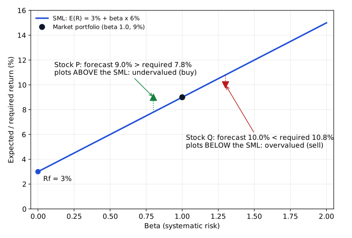
Example (, ).
- Stock P: , bought at 50, forecast price 53 plus a 1.50 dividend. Forecast ; required . P is undervalued by 1.2% and plots above the SML.
- Stock Q: , forecast 10.0%; required . Q is overvalued by 0.8% and plots below the SML.
The graph and the algebra always give the same conclusion, because the SML is the graph of the CAPM equation.
Common exam traps
- Include the dividend in the forecast holding period return. For Stock P, leaving out the 1.50 dividend gives a forecast of 6.0%, below the 7.8% required return, instead of 9.0%.
- Judging a stock against instead of against its own required return is a mistake. With a positive market risk premium, a negative-beta stock can be undervalued even when its forecast return is below .
LOS 88.i — Sharpe ratio, Treynor measure, M-squared and Jensen's alpha
Performance evaluation analyzes the risk and return of an active manager's portfolio. Attribution analysis, part of performance evaluation, looks for the sources of the difference between the active portfolio's return and a passive benchmark's return. A higher return than the benchmark proves little on its own: a portfolio with more risk (especially more beta) than the benchmark should earn more over time, so returns must be adjusted for risk.
Key concept
| Measure | Formula | Risk used | Units / reading |
|---|---|---|---|
| Sharpe ratio | Total risk | Slope of the portfolio's CAL; compare with other portfolios or the CML slope | |
| M-squared (M²) | Total risk | Percentage return of P leveraged/deleveraged to the market's σ | |
| M² alpha | Total risk | Positive if P plots above the CML | |
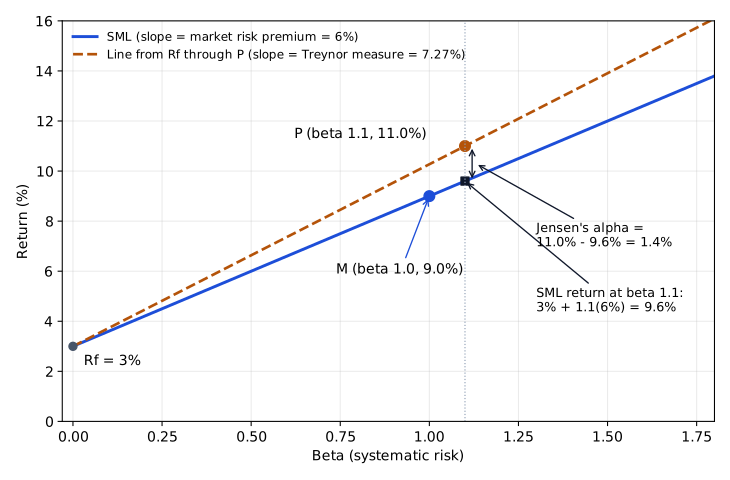
| Treynor measure | Systematic risk | Excess return per unit of beta (a slope) | |
| Jensen's alpha | Systematic risk | Percentage return above the SML |
- The Sharpe ratio can be used ex ante (expected values) or ex post (realized means and sample standard deviation). Its value is meaningful only in comparison with another portfolio's Sharpe ratio.
- M² produces the same rankings as the Sharpe ratio but is stated in percentage terms. Because , M² exceeds (M² alpha > 0) exactly when P's Sharpe ratio exceeds the CML slope. The Treynor measure and Jensen's alpha are the beta-based analogues: Treynor is a slope, and Jensen's alpha is a percentage.
- The choice of risk measure depends on whether the portfolio carries unsystematic risk. A single manager's portfolio or a concentrated holding should be judged with total-risk measures (Sharpe or M²). A well-diversified fund, such as one spread over many managers, can be judged with beta-based measures (Treynor or Jensen's alpha).
- Portfolios above the CML have higher Sharpe ratios than any CML portfolio and positive M² alphas. Portfolios above the SML have higher Treynor measures than any asset on the SML and positive Jensen's alphas.
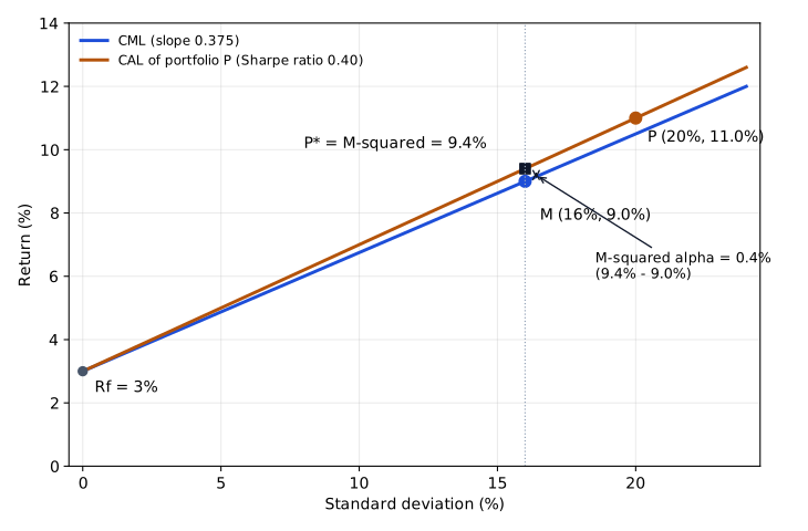
Example. , , ; , , .
- Sharpe , above the CML slope of , so P beat the market on a total-risk basis.
- M² ; M² alpha .
- Treynor , against a market Treynor measure of 6%.
- Jensen's alpha .
Example (the two families can rank funds differently). , , .
| Return | σ | β | Sharpe ratio | M² alpha | Treynor measure | Jensen's alpha | |
|---|---|---|---|---|---|---|---|
| Fund X | 12% | 24% | 0.9 | 9/24 = 0.375 | 3 + 0.375(16) − 9 = 0.0% | 9/0.9 = 10.0% | 12 − [3 + 0.9(6)] = +3.6% |
| Fund Y | 10% | 14% | 1.2 | 7/14 = 0.50 | 3 + 0.50(16) − 9 = +2.0% | 7/1.2 = 5.8% | 10 − [3 + 1.2(6)] = −0.2% |
| Market | 9% | 16% | 1.0 | 6/16 = 0.375 | 0.0% | 6/1.0 = 6.0% | 0.0% |
Fund Y wins on the total-risk measures (Sharpe 0.50 against 0.375; M² alpha +2.0% against 0.0%). Fund X wins on the beta-based measures (Treynor 10.0% against 5.8%; Jensen's alpha +3.6% against −0.2%). X has a low beta but a high standard deviation, so much of its risk is unsystematic. If X is the investor's whole portfolio, that risk matters and Y is better. If X is one small part of a well-diversified fund, its unsystematic risk is diversified away and X is better. Sharpe and Treynor values are read by comparing them with another portfolio or with the market; M² alpha and Jensen's alpha are read directly, where a value above zero means the fund beat the market after adjusting for risk.
On a graph of return against beta, P's Treynor measure is the slope of the line from through P, and its Jensen's alpha is the vertical gap between P and the SML at .
The inputs to these measures, including the expected market return (and hence the market risk premium) and betas, are estimated with error. The expected market return need not equal its historical average. Results from the models are only as good as those estimates.
Common exam traps
- Sharpe and M² use standard deviation; Treynor and Jensen use beta. Distractors often use the wrong risk measure.
- When M² alpha is asked, subtract the market return from M²; reporting M² itself is a common slip. In the example, reporting M² gives 9.4% instead of an M² alpha of 0.4%.
- Forgetting to subtract in the numerator of the Sharpe or Treynor ratio. In the example, the Sharpe ratio becomes 0.55 instead of 0.40 and the Treynor measure 10.0% instead of 7.27%.
Exam shortcuts
- M² is above exactly when the portfolio's Sharpe ratio is above the CML slope, so the sign of the M² alpha can be read from the Sharpe ratio comparison.
- Any asset with a beta of 1 has the market's required return under the CAPM whatever its total risk, so no calculation is needed for it.
Bottom line
- The CAPM, , is the equation of the security market line, whose intercept is and whose slope is the market risk premium.
- The CAPM assumes risk-averse, utility-maximizing investors, frictionless markets, a single common period, homogeneous expectations, infinitely divisible assets and competitive markets in which investors are price takers.
- The CML measures risk by standard deviation and in equilibrium holds only efficient portfolios, while the SML measures risk by beta and holds all properly priced securities and portfolios, so a single stock plots below the CML but on the SML.
- A security whose forecast return exceeds its CAPM required return plots above the SML and is undervalued, one whose forecast is below plots below the SML and is overvalued, and the difference is its expected alpha.
- With a positive market risk premium a negative beta gives a required return below , and when is below a negative beta gives a required return above .
- The Sharpe ratio and M² use total risk and suit a single manager's or concentrated portfolio, M² ranking portfolios as the Sharpe ratio does, while the Treynor measure and Jensen's alpha use beta and suit a well-diversified fund.
Quick check
Denholm Freight shares have a beta of 1.15. The risk-free rate is 2.5% and the expected return on the market is 8.5%. According to the capital asset pricing model, the required return on Denholm shares is closest to:
Show answer and explanation
Correct answer: C
The CAPM adds a beta-adjusted market risk premium to the risk-free rate. The market risk premium is the expected market return minus the risk-free rate, 6.0%.
Why the other options are wrong
- A. 12.3% multiplies beta by the full market return instead of the market risk premium: .
- B. 9.8% is simply beta times the market return (), ignoring the risk-free rate and the premium structure of the CAPM.
Key takeaway CAPM: . Subtract from the market return before multiplying by beta.
Practice Questions
A fixed-income manager holds bonds from many different issuers. After this diversification, the risk from which of the following events is most likely to remain in the portfolio?
Show answer and explanation
Correct answer: B
A recession is an economy-wide event that affects nearly all issuers at once, so its risk is systematic (market) risk and cannot be diversified away. Holding bonds of many issuers removes only unsystematic risk, which comes from events specific to one issuer.
Why the other options are wrong
- A. A downgrade after one issuer's accounting scandal is specific to that issuer. It is unsystematic risk, and its effect on a portfolio of many issuers' bonds is diversified away.
- C. A fire at one issuer's plant is a firm-specific event. Holding bonds of many issuers diversifies this unsystematic risk away.
Key takeaway Ask: does the risk come from one issuer or from the whole economy? Issuer-specific = unsystematic, diversified away; economy-wide = systematic, remains.
An analyst's CAPM-based expected return for Harwell Mining shares is 2.2 times the 10% return expected on the market portfolio. With a risk-free rate of 4%, the beta of Harwell Mining shares is closest to:
Show answer and explanation
Correct answer: A
The CAPM links a stock's expected excess return to the market's expected excess return through beta, so beta can be backed out once both excess returns are known. Harwell's expected return is .
Why the other options are wrong
- B. 2.2 is the multiple of the market's return. That multiple relates total returns, whereas beta relates excess returns over the risk-free rate.
- C. 1.8 divides the stock's excess return (18%) by the market's total return (10%) instead of by the market risk premium (6%).
Key takeaway To back out beta: . Subtract from both returns.
About 60% of Mariela Cortez's wealth is in shares of the software company she founded; the rest is in a broad mix of bonds and equity index funds. Which of the following risk-adjusted performance measures is least appropriate for evaluating her overall portfolio?
Show answer and explanation
Correct answer: B
Jensen's alpha adjusts for systematic (beta) risk only, which suits a well-diversified portfolio. Cortez's portfolio is dominated by one stock and carries a large amount of unsystematic risk, so a measure based on total risk is needed.
Why the other options are wrong
- A. The Sharpe ratio uses standard deviation (total risk), so it captures her large firm-specific risk and is appropriate for a concentrated portfolio.
- C. M-squared is derived from the Sharpe ratio and also uses total risk, so it remains suitable when the portfolio is concentrated in one holding.
Key takeaway Use total-risk measures (Sharpe, M²) for a concentrated portfolio and beta-based measures (Treynor, Jensen's alpha) for a well-diversified one.
This reading has 105 questions in the full bank. Practice all of them.
Key Takeaways
- Standard deviation is linear in the risky weight; variance is not.
- Ask: does the risk come from one issuer or from the whole economy? Issuer-specific = unsystematic, diversified away; economy-wide = systematic, remains.
- To back out beta: . Subtract from both returns.
- CAPM: . Subtract from the market return before multiplying by beta.
- Use total-risk measures (Sharpe, M²) for a concentrated portfolio and beta-based measures (Treynor, Jensen's alpha) for a well-diversified one.